1 OVERVIEW
1.1 What?
Solar radio patrol is the continuous monitoring of radio signals coming from the Sun. The Sun is a wideband radio transmitter, broadcasting over the entire radio spectrum. By the time these signals reach the Earth, they are usually rather weak (compared to a local radio station), but they can be received by a solar radio telescope, recorded, analysed and archived. Several radio telescopes are required to monitor the wide range of signals emitted by the Sun over the entire radio spectrum, and several solar radio observatories are required around the globe at different longitudes to ensure the Sun is monitored 24 hours a day.
1.2 Why?
A continuous monitoring of solar radio emissions is useful for several purposes. The first radio signals from the Sun were discovered in the latter years of WWII when John Hey investigated interference to British radar systems. The interfering signals were found to be coming from the Sun. Following the war, scientists became interested in determining the nature and type of solar radio signals, and in relating these to physical processes occurring on the Sun. The initial reason for solar radio patrol was thus to find out more about the universe in which we live, and in particular about the star that makes life on Earth possible. CSIRO scientists in Australia were at the forefront of this research, and classified the different types of solar radio activity they observed. This reason for solar radio patrol is still valid today, and solar radio data is used in combination with observations of the Sun in other spectral bands to improve and refine our knowledge of solar physics.
The second reason for solar radio patrol is to keep watch over the Sun, a variable star, because the outbursts it sometimes undergoes can affect life and equipment on the Earth and in our near space environment. We are in effect, keeping watch over our local "space weather". Although the total energy output from the Sun (most of which is infrared and visible radiation) is constant to within 0.1%, in the radio and X-ray parts of the electromagnetic spectrum the solar output can vary by up to 5 orders of magnitude (ie by a factor of 100,000). Radio bursts from the Sun may cause direct interference to communications on the Earth or in space. Background radio levels at a wavelength of 10 cm are a good indication of the overall "activity" of the Sun. Microwave frequency emissions are a good surrogate of solar X-ray activity (which affects the terrestrial ionosphere), and can also give indications of solar particle emissions. Measurements of the drift rate of certain types of low frequency solar emissions can indicate the velocity of various phenomenon through the outer atmosphere of the Sun (the corona), and can provide input to computer models to allow them to calculate the arrival time of large plasma clouds at the Earth - which may then go on to cause geomagnetic storms, affecting terrestrial communications, navigation, long pipelines and power grids. Continuous solar radio patrol is thus very desirable for societal and economic reasons.
1.3 How?
Solar radio patrol may be carried out from the surface of the Earth from radio observatories equipped with a variety of radio telescopes. Multiple telescopes are required to cover the large frequency range of solar emissions, and to provide a range of different displays for interpretive purposes.
|
THREE REASONS FOR SOLAR RADIO PATROL
RADIO FREQUENCY INTERFERENCE The Sun is a broadband radio transmitter. Solar radio bursts can exceed the background solar radio emission by several orders of magnitude. Solar radio emissions can cause interference to man-made electromagnetic systems (eg radio and radar). It is often useful to know that interference comes from the Sun rather than from an equipment problem or from another man-made source. EQUIPMENT CALIBRATION The background solar radio emission is a relatively slowly changing source that can be observed by most antennae, irrespective of where they are on the globe or out in space. If the intensity of this radio emission is known accurately, then it can be used by anyone as a source to calibrate equipment. SPACE WEATHER PREDICTION Different physical processes occurring on the Sun produce different types of radio emission. These can be used to make predictions of the effect of solar activity on the near space environment surrounding the Earth. |
2 EMISSIONS
2.1 Radio Waves
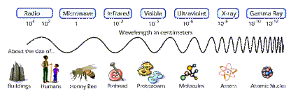
Radio waves are a form of electromagnetic energy. Other forms are infrared, visible, and ultraviolet radiation. X-rays and gamma rays are also forms of electromagnetic radiation. The difference between these different types of radiation lies in their frequency and wavelength.
In the above diagram microwaves are indicated separately from radio waves, but in fact microwaves are normally regarded as part of the radio spectrum.
Radio waves have the lowest frequency and longest wavelengths of all the different types of electromagnetic energy. The relationship between wavelength and frequency is given by the formula:
where
λ is the wavelength in metres
c is the speed of light (3 x 10⁸ metres/sec in a vacuum)
f is the frequency in Hertz
2.2 The Radio Spectrum
The radio spectrum is broken down into various frequency bands:
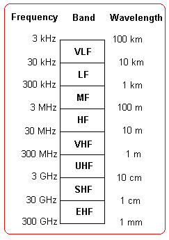 |
where the designations are:
LF Low Frequency MF Medium Frequency HF High Frequency VHF Very High Frequency UHF Ultra High Frequency SHF Super High Frequency EHF Extremely High Frequency Because the Earth's ionosphere, a region of the Earth's upper atmosphere above about 80 km, which is weakly ionised, will not allow radio signals below a frequency of about 5 to 20 MHz to pass through, radio astronomy is normally only concerned with the VHF, UHF, SHF and EHF radio sub-bands. Frequencies above 20 to 50 GHz are also absorbed strongly by components of the Earth's atmosphere (eg oxygen and water vapour), and telescopes that operate above these frequencies are often located on high mountain tops.In general, solar radio astronomy makes use of the radio spectrum from about 20 MHz to 20 GHz. This corresponds to wavelengths from 15 metres down to 15 millimetres. |
Microwave is a term that was historically employed for signals with wavelengths less than one foot (30 cm), and this region has been subdivided into letter bands. However, there are several designations for microwave bands. Two of these, which we shall call traditional and new, are given below. The traditional was devised during WWII, whereas the new is more recent.
   Traditional  f range (GHz)       New   f range (GHz)
       L          1 - 2              D       1 - 2
       S          2 - 4              E       2 - 3
       C          4 - 8              F       3 - 4
       X          8 - 12             G       4 - 6
       Ku         12 - 18            H       6 - 8
       K          18 - 27            I       8 - 10
       Ka         27 - 40            J       10 - 20
       V          40 - 75            K       20 - 40
       W          75 - 110           L       40 - 60
       mm         110 - 300          M       60 - 140
       sub-mm       >300
2.3 The Sun as a Radio Transmitter
Any time charges are accelerated or decelerated, electromagnetic energy such as radio waves are produced. In matter, electrons carry negative charge, and protons carry positive charge (ions, which can have an excess or deficiency of electrons, may carry positive or negative charge).
In normal matter, atoms are electrically neutral (having neither positive or negative charge - because they have an equal number of protons and electrons). However, in metals, electrons are free to move around the lattice of positive ions. If a changing electric field is applied to a metal or other conductor electrons may be accelerated, and radiate radio waves (e.g. in the conducting parts of an antenna).
In space there are not too many large pieces of metal, but material in stars and in the interplanetary and interstellar medium is in the form of plasma, where, although electrical neutral as a whole, the electrons and ions are not tightly bound to one another and can move around within the plasma (just as electrons can move around within a metal).
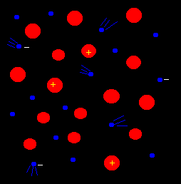 | In this representation of a plasma, electrons are shown as small blue spheres moving around the larger (red) positive ions. Because the ions are several thousands time more massive than the electrons, they move much more slowly. The electrons on the other hand respond rapidly to electric and magnetic fields, and are responsible for most of the radio emission from a plasma as they accelerate or decelerate. There are many ways in which this can occur. |
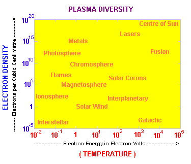
| Plasmas can be characterised by their temperature and their density (remember that the ion density must be equal to the electron density to result in a plasma that is electrically neutral overall). The diagram opposite shows the temperature and density of various plasmas from the Sun to the Earth. |
|
Any body which is hot, such as the Sun, will emit what is called thermal radiation, simply by virtue of its high temperature. In this case the electrons can be thought of as oscillating (in what we call simple harmonic motion) around a small area in the plasma (this also happens in hot gases, the atoms themselves oscillating). Different electrons or ions (or atoms) oscillate at different frequencies, producing a spectrum of emission called black body radiation. This emission has a peak frequency or wavelength (where the maximum energy emission is concentrated) which is dependent upon the temperature of the plasma or gas.
The surface of the Sun or photosphere, is where the vast majority of solar energy is emitted into space. Most of this energy is in the form of visible light and infrared radiation. However, a small fraction of the radiation is emitted as radio waves. The corona, although it has a much lower density than the photosphere, is at a much higher temperature, and predominates in the low frequency radio spectrum, in contrast to the visible spectrum where the small glow of the corona is totally overwhelmed by the light from the photosphere, except where this is occluded by the moon in a total solar eclipse.
Non-thermal radiation occurs from other electrons motions, including motions around magnetic fields. The various types of this radiation from the Sun are discussed more fully below.
2.4 Time and Frequency
Radio emissions from the Sun vary with time, and they vary with frequency. To completely monitor the radio output from the Sun we need to keep a continuous watch (for variations with time) over a very large frequency range, from about 20 MHz to 20 GHz.
We find that different frequencies are emitted from different altitudes in the corona and chromosphere, and also that different processes occurring in the Sun's atmosphere emit radio signals at different frequencies. We can often use the variation with altitude to follow an ejection of material from the Sun, as it rises from low to high altitudes, and compute a velocity of motion through the solar atmosphere.
Different processes also show different time signatures, and these can be useful in determining what is going on in the solar atmosphere, and whether it is going to produce a significant effect on the Earth (ie is an event likely to be "geoeffective").
2.5 Solar Radio Signals
The Sun is what we call a broadband emitter. That is, it gives off radiation over a very wide frequency range. At the Earth we measure this emission with a unit called the Solar Flux Unit or SFU, where:
Initially we can break down solar radio emission into three parts: the quiet (or background) component, the slowly varying component, and the burst component.
The Quiet Component
The quiet or background component of the solar radio emission is by definition the component that remains when all other variable components have been eliminated. This occurs around the time of sunspot minimum, although we are still not certain that the Sun does indeed return to exactly the same state, radio wise, each solar cycle - at the moment we assume this. Our equipment is simply not stable enough over an 11 year period to assure us of this. Thus we assume that the quiet component varies only with frequency (i.e. not with time). It has a flux density of about 10 SFU at a frequency of 200 MHz, and increases to 500 SFU at a frequency of 15,000 MHz.
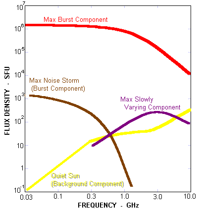
The above diagram shows how the quiet component of the Sun varies with frequency. It also shows the approximate maximum values obtained by both the slowly varying component and the burst components.
The Slowly Varying Component
The slowly varying component is a radio emission from the chromosphere and corona around and above active solar regions. It shows a strong correlation to the amount of plage observed in H-alpha images, and thus is also highly correlated with sunspot number. The slowly varying or S-component of solar radio emission shows a peak around a frequency of 3 GHz, which corresponds to a wavelength of 10 cm. Thus measurements of solar radio flux around 3 GHz are often referred to as the 10 centimetre solar flux.
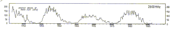
The slowly varying component shows a variation typically on two time scales. The first, of approximately 27 or 28 days, is the rotation period of the Sun at mid-latitudes. This variation is due to the uneven distribution of plage with solar longitude. As an area of intense and extensive plage rotates onto the visible disc (as seen from the Earth), the S-component increases. A small plage area may grow and decay within a day. A large area may persist for several solar rotations, This process will also produce random fluctuations in the S-component on a time scale of less than one solar rotation.. The second and much longer principal variation in the S-component is around 11 years, in time with the sunspot cycle, as overall plage area waxes and wanes. Over one solar cycle, the slowly varying component at 3 GHz may vary from 0 to 250 SFU. Typical variations over a few decades are shown in the graph below.
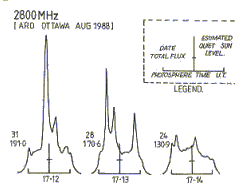
Because the slowly varying component is produced by specific regions on the Sun it shows a significant variation over the solar disc. If a radio telescope has sufficient resolution, a scan across the disc will show the "hot" spots producing this component. The diagram below is a one dimensional scan from east to west across the Sun. The peaks in the S-component can be clearly seen.
The Burst Component
The burst component is a transient radio emission from the Sun associated with localised and often explosive energy releases in the solar chromosphere and corona. At lower frequencies (20 to 200 MHz), or what are often referred to as metre wavelengths, the burst component may increase the total solar output by up to six orders of magnitude, with this increase lasting anywhere from seconds to hours. Thus, the quiet Sun output of about 1 SFU at 80 MHz may increase to one million SFU when a major burst occurs.
The occurrence frequency of bursts varies enormously over the ~11 year sunspot cycle. At times of sunspot minimum one may wait weeks or even months between small solar radio bursts, whereas they may occur several times a day during times of maximum activity. Not only does the frequency of bursts increase, but the intensity of bursts generally increases at the same time.
At the higher microwave frequencies (e.g. 20 GHz), the maximum intensity that the burst component can attain is limited to about 20,000 SFU by a process called synchrotron self absorption.
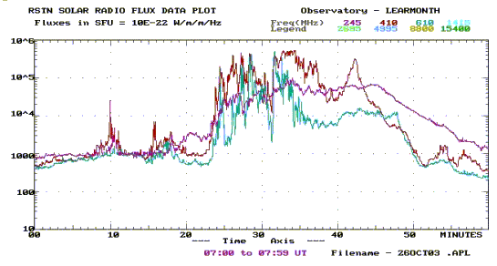
An example of a long duration high intensity multifrequency solar radio burst is shown below. Note that the burst started before the start of the plot, as the flux values are then well above the quiet Sun values for the three frequencies plotted.
2.6 Solar Radio Emission Processes
Having discussed the different components of solar radio signals, we need to say a little bit about how these signals are produced. That is, what physical processes occur on the Sun to produce these signals.
If you remember we previously divided radio emissions into thermal and non-thermal emissions. The quiet component is mainly a result of thermal emission. That is, it is produced as a result of oscillating charges, vibrating because they are at a high temperature.
On the other hand the burst component, is non-thermal, and it is produced on the Sun through one or more of four main mechanisms:
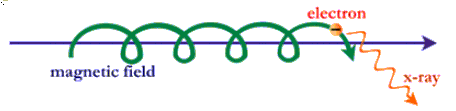
This is a German word that means "braking radiation". It was first used to describe the production of X-rays in the early experiments of and leading on from Roentgen. In an X-ray tube, electrons from a cathode (negative element) were accelerated toward an anode (positive element) by a potential of tens of thousands of volts. When the electrons reached the anode they were brought to a very rapid stop as they smashed into the atoms making up the anode. This violent deceleration of negative charge produced high energy X-rays. The radiation itself was thus called bremstrahlung.
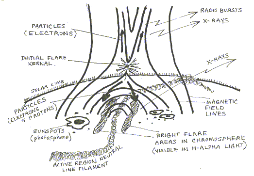
In the solar case, a flare kernel high in the corona starts where magnetic field lines snap and then reconnect in a lower energy configuration. Electrons are accelerated away from this point, some down toward the chromosphere and some higher into the corona. Eventually they will collide with an atom, suffering large decelerations and emitting radio energy (their energy of motion, or kinetic energy is exchanged for electromagnetic energy).
Bremstrahlung radiation is a broadband radiation and is believed to be responsible for some of the microwave radiation associated with optical and X-ray flares. In fact it is believed that the same electron population (although not exactly the same electrons) are responsible for both the radio and the X-ray emissions observed during a flare.
Plasma Radiation
Plasma is the fourth state of matter. It consists of equal numbers of positive and negative charges, and so overall is electrically neutral. The solar corona is a highly ionised plasma. Because the individual charges are free to move around in the plasma, it sometimes occurs that the negative charges are partially separated from the positive charges and so there is a lack of local neutrality.
Now because opposite types of charge attract each other, a force exists which tends to bring the two regions of charge back together. So the negative and positive charge centres are accelerated toward each other. However, because plasma is mostly empty space, the charges overshoot. Then they experience a force in the opposite direction to bring the charges back again toward a situation of neutrality. So there is an oscillation of charges for a little while until bulk neutrality of the plasma is achieved. Now because electrons are only about 1/2000th the mass of the protons in a hydrogen plasma, it is the electrons that do most of the moving in this oscillation. And as oscillation involves acceleration and deceleration, electromagnetic radiation (radio waves) will be emitted.
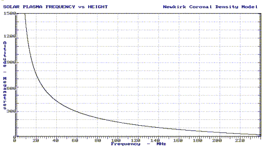
The frequency of plasma radiation is proportional to the square root of the electron density. In the corona, at a temperature of a few million degrees, most of the hydrogen will be fully ionised, and thus the electron density will be equal to the total species density. We expect this density to decrease as the distance from the photosphere increases (i.e. decreasing atmospheric density with altitude). We generally use a coronal density model developed by Gordon Newkirk, and from this we can calculate the variation of plasma frequency radiation with altitude above the photosphere. The graph below shows the result.
|
CORONAL ELECTRON DENSITY (1) The simplest model assumes an isothermal corona (ie uniform temperature) and that gravity remains constant throughout the corona. The resulting formula for the electron density is:
where No is the extrapolated density at the photosphere (not real) β = 1/H where H is called the scale height of the atmosphere h is the height above the photosphere. (2) The Newkirk model assumes that gravity decreases with altitude (as it does). This gives a formula that more closely matches the real behaviour of the solar corona:
where r = h + 1 PLASMA FREQUENCY
The natural resonance frequency of a plasma is given by:
where e = 1.6x10⁻¹⁹ Coulomb is the charge on an electron π = 3.14159..... me = 9.1x10⁻³¹ kg is the mass of an electron ε = 8.85x10¹² Farad/metre is the plasma permittivity |
We should note that the corona of the Sun is a very active and dynamic atmosphere, and that the Newkirk model can at best describe only some average electron density. Still, using this model we can make an estimate of the propagation speed of shock waves through the solar atmosphere. Practical use of these formula is illustrated in section 4.4 which discusses analysis of various solar radio emissions.
Cyclotron Radiation
When low energy electrons (with speeds no more than about 10% the speed of light) encounter regions of magnetic field they are constrained, by the magnetic field, to move in circles around the magnetic field. This is because the force they experience is at right angles to both their velocity and the magnetic field direction.
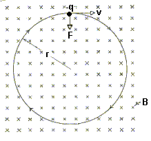
Here the magnetic fields are shown as going into the plane of the diagram. The direction of motion is shown by the velocity vector v for a negative charge (-q) like an electron. The centripetal force F is the force acting on the moving electron due to the magnetic field. This constrains the electron to move in the circle of radius r. If the electron has a component of velocity perpendicular to the plane of the circle, then its overall motion is a helix, as shown below.
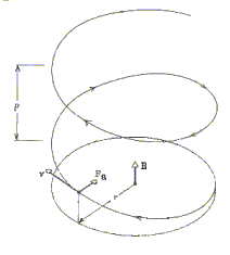
The radiation emitted by electrons exhibiting this type of motion is called cyclotron or gyro radiation. It is a narrow bandwidth radiation and rather directional, being emitted in a cone. The frequency of the radiation, called the cyclotron frequency or gyrofrequency is given by:
When the energy of circling or gyrating electrons becomes larger and their speed increases to a substantial fraction (>10%) of the speed of light (we then say they have become relativistic), the nature of the radiation they emit also changes. It becomes broadband in nature. That is, the frequency of the emitted radiation is spread over a wide or broad frequency spectrum. It can range from radio to X-rays. Synchrotron radiation is a very significant radiation throughout the universe.
The following images show the synchrotron radiation from the Crab nebula at four different wavelengths over the entire electromagnetic spectrum.
| RADIO OPTICAL |
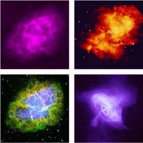 | INFRARED XRAY |
|
POINTS TO REMEMBER
1 Different frequency emissions can be due to different emission mechanisms. High microwave frequency emission is invariably due to synchrotron radiation, as electron densities in the corona are not high enough to support gigahertz plasma radiation. 2 Different frequency emissions can be due to the one emission mechanism with different conditions (eg cyclotron radiation at different frequencies is due to a difference in magnetic field strength, & plasma radiation at different frequencies is due to a difference in free electron density which can then be related to height in the corona) 3 Spectral burst morphology (form) can generally allow us to distinguish what is occurring. The variation of intensity with both frequency and time is necessary to sort out solar radio emissions. |
3 EQUIPMENT
3.1 Types of Solar Radio Telescope
There are several different types of solar radio telescope that have been built, each to serve to a different purpose. The three main types are:
A radiospectrograph is a radio telescope that continually sweeps over a specified range of frequencies. The output produced is a rectangular (moving) map where a grey scale or colour is used to indicate flux density, and the two axes of the map are frequency and time. A spectrograph is very useful to quickly identify different spectral emissions from the Sun, and to make measurements of these.
A radioheliograph is generally the most complex of solar radio telescopes, and is used to produce an image, or spatial picture of solar radio emissions. A simple type of this instrument may resolve the Sun in only one direction, showing how radio emission varies across the east-west axis of the Sun. A more comprehensive radioheliograph will produce a two dimensional image of the Sun, just like (although generally with lower resolution) a visible image or photograph. Radio heliographs are very large, expensive and costly to run and maintain, and are rarely available for routine continuous solar patrol. This is not to say however that they are not useful. One particularly complex type of solar emission (type IV bursts) can only really be truly identified and characterised using a radioheliograph.
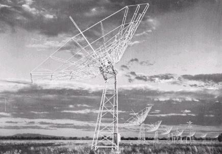
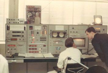
The photo above shows a few of the 96 antennae built by CSIRO for the Culgoora Radioheliograph. These antenna lay on the circumference of a 3 km circle. They would each track the Sun across the sky during the day, and allowed the production of low resolution images showing material moving away from the Sun (or at least the radio emission from the moving material). The control console of the radioheliograph is shown below.
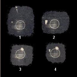
Below, four initial images from this radioheliograph show solar radio emission at 80 MHz from different places in the solar corona. These were observed during a five minute time frame on 2 September 1967.
We shall not discuss radioheliographs any further.
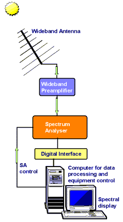
3.2 Discrete Frequency Radio Telescopes
A single or discrete frequency radio telescope is also referred to as a radiometer. A simplified outline diagram of such a radiometer is shown below.
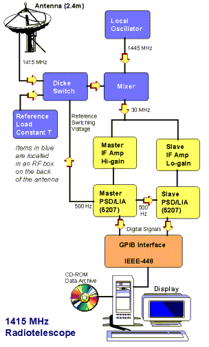
This type of radio telescope comprises an antenna to collect the signals from the Sun. Since these signals are only a very small fraction of a microwatt, they need to be amplified so that they can be plotted on a chart recorder, or digitised for ingestion by a computer which then uses software to plot the output of the telescope versus time.
However, it is not possible to simply amplify the signal at the received frequency, and the above diagram illustrates some of the design features that must be built into a radiometer to ensure a relatively noise free and stable output.
First, amplifiers are a lot easier to construct at low rather than high frequencies. So the radio frequency signal from the Sun, at 1415 MHz is 'downconverted' to an 'intermediate' frequency of only 30 MHz where most of the signal amplification takes place. As amplifier gain tends to change with the temperature, it is essential to maintain this piece of electronic circuitry, which can provide an amplification in excess of 10 million times, in a temperature controlled environment (typically controlled to within one degree Celsius).
The downconversion process is carried out in a component called a mixer, which 'beats' the incoming signal frequency of 1415 MHz, against a reference signal generated by a stable local oscillator at 1445 MHz. The output of the mixer will consist of both a 'sum' and a 'difference' frequency of 2860 and 30 MHz respectively. The difference frequency of 30 MHz is selected for by a filter to pass only this frequency along to the 30 MHz intermediate frequency (IF) amplifiers.
The reason for two rather than one IF amplifiers lie in the dynamic range of the solar signal. It is difficult to construct a single amplifier which has a linear response over a dynamic range of more than about 1000. By linear we mean that the output of the amplifier can be expressed by the equation:
Thus, when we require linear amplification over more than three orders of magnitude (i.e. more than a factor of 1000), we need to employ two (or more) amplifiers, each of which is used for a particular amplitude of signal. The high gain amplifier might be used to deal with solar signals from 1 to 1000 SFU, and the low gain amplifier is used to deal with signals from 1000 to 1 million SFU. In this way, we can ensure reasonably accurate measurement and recording of solar emissions from one to a million solar flux units.
The computer at the output of the radiotelescope knows that when the high gain amplifier is saturated (i.e. its output has reached 1000 SFU), it is time to switch over and use the output of the low gain amplifier.
Even with this duplication of amplifiers, it is sometimes necessary to provide a software correction to each amplifier to ensure that the resultant output is totally linear. This is done through a process referred to as a linearity calibration, and will be discussed later.
There is one further complication in a practical radiometer which we have not yet discussed, and this is related to high gain amplifiers. With all amplifiers, and particularly with high gain amplifiers, we have the problem of noise. Noise is defined as an extraneous signal which appears in any electronic circuitry alongside the desired or wanted signal. Noise is generated in most electronic components (e.g. resistors and transistors). Low frequency noise or amplifier drift is also caused by component ageing and component temperature changes. High frequency noise is simply an inherent part of the amplification process (like death and taxes, something that cannot be avoided, although we can try to minimise it).
To reduce noise and drift in the radiometer, we use what is called a Dicke loop, after the Princeton physicist Robert Dicke, who devised the principle at the end of the second World War. Instead of simply amplifying the signal we collect from the Sun by the antenna, we switch the input of the radiotelescope receiver between the antenna and a 'constant temperature load' which is a very stable resistor maintained at an elevated and strictly controlled temperature in a small 'oven'. This load generates a constant amount of radio frequency noise - by virtue of its temperature. This switching takes place several hundred times each second (500 Hz in the above diagram). The switching is done by a component called a Dicke switch.
The output of the receiver is switched in synchronism with the Dicke switch in a device called a phase synchronous detector or lock-in amplifier. The output of this PSD/LIA gives the difference between the load noise and the solar signal. In computing this difference the LIA reduces the noise produced by the preceding amplifiers, and a cleaner output signal is obtained.
We can make an analogy to measuring the mass of an object using a beam balance rather than a spring balance. When we use a spring balance (which would be equivalent to using a straight amplifier with no Dicke loop), we rely on the properties of the spring, which can change. When we use a beam balance, we are comparing the object we wish to measure with a set of standard masses. In other words, the beam balance is performing a comparison measurement, and has a greater accuracy (dependent on the accuracy of the set of standard masses) than where we rely on the properties of a spring.
Finally, the outputs of the two PSD/LIA's are digitised and fed to a computer over a General Purpose Interface Bus. A software program will ingest this signal, convert it into the appropriate units, display it for the radioastronomer to see, and store it for archive purposes. A graphical display output for a solar radiometer, showing a solar burst, is shown below.
In summary, a solar radiometer is a single or discrete frequency radio telescope that can be well calibrated to provide an accurate linear output of the observed source over a wide dynamic range.
3.3 Swept Frequency Radio Telescopes
One of the disadvantages of a single frequency radiometer is that you have no knowledge of what is happening on adjacent frequencies. As solar processes generally produce signals that have a wide frequency bandwidth, and that drift in frequency over short and long time intervals, it is often highly advantageous to have a radiotelescope that presents you with a spectral display. That is, one that shows signal intensity as a function of both frequency and time. Such a radiotelescope is generally called a radiospectrograph. A block diagram of such a telescope is shown below.
The special features that this type of radio telescope must display are a wide bandwidth antenna and preamplifier.
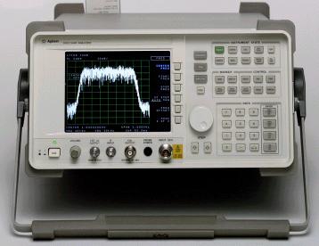
The radiospectrograph is often built around a commercial spectrum analyser, which is a special receiver that has the ability to sweep over a large range of frequencies in a relatively short time. A picture of such a commercial unit is shown below.
A wideband preamplifier is required before the input of the analyser to increase the overall sensitivity to a level sufficient to detect small solar signals. The spectrum analyser is usually set to work as a logarithmic amplifier in order to cope with the wide amplitude of signals from the Sun.
The output of these analysers is often already available in digital form that can be fed straight to a computer via a General Purpose Interface Bus (GPIB).
The spectrum analyser also needs to be set up to scan over the required frequency range with a specified bandwidth, scan rate, and some other parameters. This can be done manually, or over a control bus (often the same GPIB which is used for output data transfer) from a controlling PC.
A typical frequency scan might be from about 20 to 200 MHz. Sometimes this is done in two or more bands in order to obtain higher frequency resolution and/or increase the frequency coverage. A scan over this frequency range will typically take from 1 to 5 seconds. For each scan, around 500 data points are passed from the analyser to the PC. These represent the logarithmic amplitudes of the signal received at each of 500 frequencies sampled (usually uniformly) over the frequency range. A display of a solar radiospectrograph is shown below.
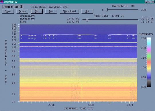
This spectrograph employs two spectrum analysers to sweep two frequency bands, the lower one from 25 to 75 MHz and the upper one from 75 to 180 MHz. This is necessary because it is not always possible or desirable to build one antenna to cover such a large frequency bandwidth.
In this display, the horizontal axis represents time and the vertical axis represents frequency. The intensity of the received signal at a given time and frequency (i.e. for a specific pixel of the video display) is represented by a colour. The colour bat to the right of the main display represents an 8-bit logarithmic intensity measured by and output from the spectrum analysers to the data processing and display computer. Being 8-bits, this amplitude scale thus has a range from 0 to 255.
For a number of reasons, a spectrograph cannot easily be accurately calibrated in terms of solar flux units as is done in the case of a single frequency radiometer. The amplitude units are then regarded as a relative intensity scale.
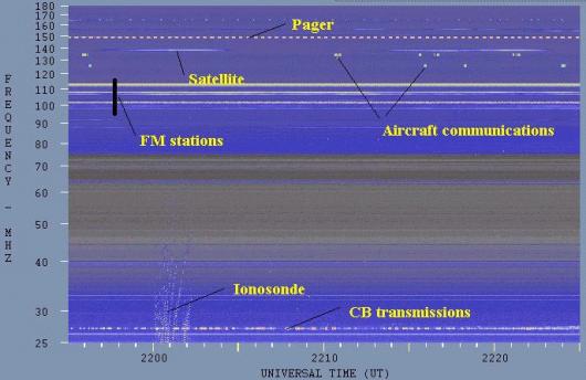
There are no solar signals present on the above display. However, a lot of man-made signals can be seen. Because man-made signals are generally narrow band in nature, they appear as either continuous or intermittent horizontal lines on this type of display. Continuous horizontal lines usually indicate broadcast transmissions (e.g. from FM radio stations), whereas broken or intermittent horizontal lines indicate two way communications (e.g. between aircraft and ground controllers).
Unfortunately, radio astronomy must share the radio spectrum with many other users, and interfering signals are always going to be present in spectral displays (except possibly for a radio observatory located on the far side of the moon).
3.4 Antennae
An antenna is a device to collect radio energy. Used as part of a solar radiotelescope, it is of course collecting solar radio energy. The type of antenna used is dependent of the type and frequency of radiotelescope.
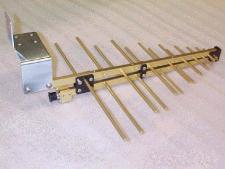
For low frequency radiometers, a yagi antenna may be employed.
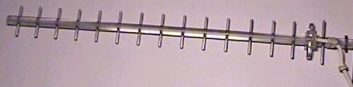
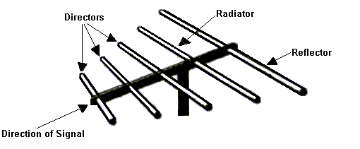
A yagi consists of a long central boom to which are added various smaller elements at right angles to the boom. There are three types of elements. Second from the right is the only active or driven element, sometimes called the radiator. This is the element from which the desired signal is extracted and fed to the receiver by a feedline (in this case a coaxial cable). The element to the right of the driven element is called a reflector. Its function is to reflect the signal back to the driven element. The 14 elements to the left of the driven element are called directors. Their function is to direct the signal to the driven element. The boom points to the desired signal source, which here is to the left of the image. The driven element is one half wavelength long, the reflector is about 5% longer. The directors are progressively a little shorter than one half wavelength. A labeled diagram of a Yagi antenna is shown below indicating the various elements.
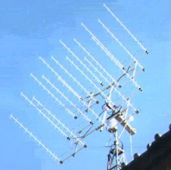
This type of antenna has a small frequency bandwidth and can thus only be used for a single frequency radiometer. To obtain more signal (ie increase the antenna gain), sometimes several yagis are stacked together in an array.
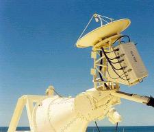
At microwave frequencies, a parabolic antenna is generally used for a solar radiotelescope. The parabolic dish simply acts as a reflector, independent of frequency, that collects the radio signals falling on the entire area of the dish and focusing them to the focal point of the antenna. This generally lies some distance above the centre point of dish.
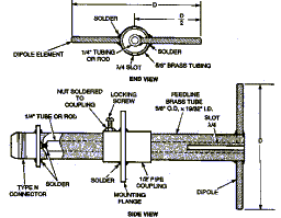
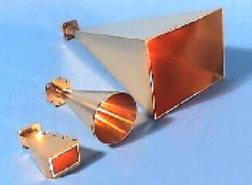
Another antenna, called a feed antenna, or feed, must be placed at the focal point to convert the signals focused at this point to an electrical signal which is then conveyed to the receiver (or a preamplifier placed before the receiver). The simplest type of feed is a (half-wave) dipole. This may be used for the lower microwave frequencies, but a horn type feed (called a feed horn) is generally used at the higher microwave frequencies. The dipole would generally be fed by a coaxial cable, whereas a feedhorn would be connected to a waveguide.
 |
 |
The 2.4m diameter parabolic antenna shown on the previous page has four different feed antennas clustered around the focal point of the dish. Two of these are dipoles and two are feedhorns. The fours frequencies thus supported are 1415, 2695, 4995 and 8800 MHz. The dipoles are used for the two lower frequencies.
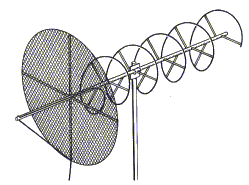
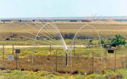
For a radiospectrograph a wideband antenna is required. Two types of such antennae are the helical antenna or helix and the log-periodic antenna. The helix will operate over a two to one frequency range, whereas a log-periodic antenna will function over a ten to one frequency range.
 |
 |
These antennas may be used as stand alone antennas, they may be stacked in arrays to increase the gain (with a consequent reduction in beamwidth), and they may be used as feed antennae with a parabolic dish.
All of the above antennae have narrow beams and thus must be made to track the Sun as it moves across the sky during the day. The tracking mount may be an equatorial mount, which usually needs a declination adjustment each day, and the motion in right ascension or hour angle can be achieved by a synchronous motor that drives the antenna across the sky at a solar rate.
It is also possible to use an elevation-azimuth mount (also known as an alt-az mount), but a computer must be used to compute the elevation and azimuth of the Sun during the day and send the appropriate commands to the tracking motors. Analog sensors, or digital encoders are used to sense the actual position of the antenna at any time and provide this information as feedback to the controller.
 |
 |
At low frequencies, an omnidirectional wideband antenna can be used. This has the great advantage of not having to track the Sun. One such antenna is a semi-bicone. Although it is not strictly omnidirectional, it has nulls along the axis of the cones, and if these are orientated north-south, the Sun at mid-latitudes, will never appear in these null zones.
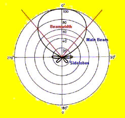
Antenna Beamwidth
| The beamwidth of an antenna is basically the angle over which it responds to signals. Technically it is defined as the angle over which the antenna drops from a maximum to half this maximum. Of course, the antenna will respond to strong signals outside the beamwidth, but with reduced gain. All antennas also have "sidelobes" where the antenna response is reduced but still susceptible to interfering signals that are "off axis" or substantially away from the direction to which the antenna is pointing. The diagram opposite shows the "polar response pattern" of a typical parabolic antenna, showing the main beam, the angular beamwidth, and the sidelobes. |
 |
The beamwidth of a parabolic antenna is dependent on both its diameter and the wavelength of the signals it is receiving. The formula to compute the beamwidth is given by the simple equation:
ANTENNA BEAMWIDTH (in degrees) Antenna Frequency (MHz) Diam(m) 20 50 100 200 500 1000 2000 5000 10000 1.0 ** ** 171.89 85.94 34.38 17.19 8.59 3.44 1.72 1.5 ** ** 114.59 57.30 22.92 11.46 5.73 2.29 1.15 2.0 ** 171.89 85.94 42.97 17.19 8.59 4.30 1.72 0.86 2.5 ** 137.51 68.75 34.38 13.75 6.88 3.44 1.38 0.69 3.0 ** 114.59 57.30 28.65 11.46 5.73 2.86 1.15 0.57 3.5 ** 98.22 49.11 24.56 9.82 4.91 2.46 0.98 0.49 4.0 ** 85.94 42.97 21.49 8.59 4.30 2.15 0.86 0.43 4.5 ** 76.39 38.20 19.10 7.64 3.82 1.91 0.76 0.38 5.0 171.89 68.75 34.38 17.19 6.88 3.44 1.72 0.69 0.34 5.5 156.26 62.50 31.25 15.63 6.25 3.13 1.56 0.63 0.31 6.0 143.24 57.30 28.65 14.32 5.73 2.86 1.43 0.57 0.29 6.5 132.22 52.89 26.44 13.22 5.29 2.64 1.32 0.53 0.26 7.0 122.78 49.11 24.56 12.28 4.91 2.46 1.23 0.49 0.25 7.5 114.59 45.84 22.92 11.46 4.58 2.29 1.15 0.46 0.23 8.0 107.43 42.97 21.49 10.74 4.30 2.15 1.07 0.43 0.21 8.5 101.11 40.44 20.22 10.11 4.04 2.02 1.01 0.40 0.20 9.0 95.49 38.20 19.10 9.55 3.82 1.91 0.95 0.38 0.19 9.5 90.47 36.19 18.09 9.05 3.62 1.81 0.90 0.36 0.18 |
3.5 Amplifiers
The amplifiers and preamplifiers that are used in radioastronomy have essentially the same design as radio frequency amplifiers used in radio communication equipment. The essential characteristics for radio astronomical purposes are low noise, wide bandwidth and high stability.
Low noise preamplifiers are frequently used before the main receiver to ensure high system sensitivity. The preamplifiers may have one or more transistors (often GaAs transistors for low noise) or may use integrated circuit amplifiers.
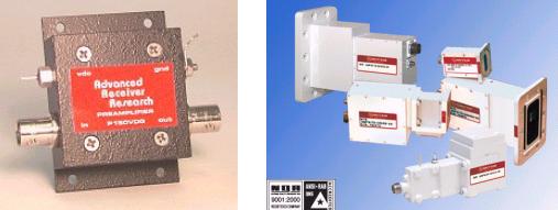 |
The circuit diagram for a single transistor low noise broadband preamplifier is shown below together with the constructional details for the unit.
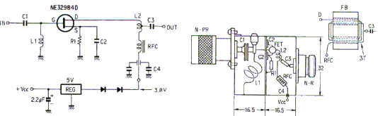
This amplifier employs a low noise Gallium Arsenide (GaAs) field effect transistor (FET) for low noise performance, and a bifilar wound inductor (L2) to ensure wide bandwidth.
Preamplifiers of these types are built into solid metal enclosures to ensure immunity to stray RF signals and to help keep down circuit losses through radiation of the signal.
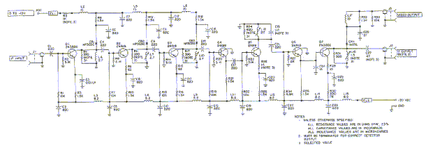
Preamplifiers are designed to operate at the signal frequency. However, most of the radiotelescope amplification takes place at the intermediates frequency. This is normally below 100 MHz, and 30 and 70 MHz are common IF frequencies. Gains of 1 to 100 million are typical in the IF amplifiers. To obtain these types of gains, several stages of amplification are required. This may be performed by discrete transistors or a number of integrated circuits. For many purposes the IF amplifier is required to provide linear amplification, although some, particularly for spectrographs, may require a logarithmic output.
The circuit diagram of a 30 MHz IF amplifier used in the discrete frequency radiotelescopes at Learmonth Solar Observatory is shown below.
3.6 Output Displays
The output of a radiotelescope is displayed so that humans can interpret the signal. A single frequency radiometer output is a time varying amplitude, and is generally plotted as a simple graph of signal intensity versus time.
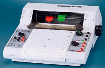
Before the widespread use of computers, it was common to plot this signal using a device called a chart recorder in which a pen would move according to the intensity of the signal and draw a line on a long strip of paper moving beneath the pen. The chart recorder shown below has two pens, one which draws a red line, and the other a green line. Thus the output of two radiometers, or of one radiometer with different output sensitivities, may be plotted on the one chart.
A chart recorder plot of the integrated solar emissions from 30 to 80 MHz is shown in the graph below. A series of type 3 solar radio bursts can be seen.
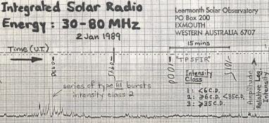
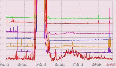
Chart recorders find very limited use these days, because of the archive problem. It is generally much simpler to digitise the output of a radiotelescope and feed it to a computer, which can not only display the output in a variety of forms for immediate perusal and measurement, but which can also archive the data in files that can easily be duplicated and made available to others. When a hard copy is required of a particular event, the data can be formatted and printed out graphically on a computer printer. The following screen dump shows multiple single frequency plots between 18 and 28 MHz recorded at the University of Florida Radio Observatory. A very large solar burst occurred around 16:50 UT and has caused all the traces to saturate. (This indicates the need for either a logarithmic scale or multiple linear scales of different sensitivity when observing the Sun).
A solar radio spectrograph has a totally different type of plot. The plot is generally in the form of a frequency-time 2D map in which signal intensity is indicated either by a grey scale or a colour scale. Although radiospectrographs have used paper charts (similar to facsimile machines) in the past, today, computers and their associated monitors are used to present such outputs.
The following radio spectrograph display is from an observatory in Athens, Greece, and it show fine detail in a group of type III bursts. The horizontal scale is time, and the fiducial marks are separated by 25 seconds in this axis.
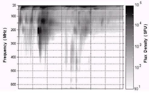
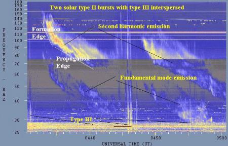
The next radiospectrograph display is from Learmonth Solar Observatory and shows type II emission.
4 OPERATIONS
4.1 Monitoring
The reasons for continuous solar radio patrol have already been discussed in section 1. However, a single observatory can only monitor the Sun between the hours of sunrise and sunset. A network of observatories is required if a continuous watch on the radio Sun is to be maintained. It is also desirable that each station has some overlap to cope with equipment outages and weather problems. Although radio observation is not limited by weather to nearly the extent of an optical observatory, heavy clouds will attenuate the higher microwave frequencies, and heavy rain may attenuate signals all the way down to 1 GHz.
Space based observations can get around the problem of clouds and the diurnal cycle - a satellite in geosynchronous orbit only experiences short eclipses due to the Earth's shadow for a few days around the equinoxes. However, unlike optical telescopes, radio telescopes require very large structures which are very expensive to build and launch into space. Radio telescopes in space are also subject to a very intense radio frequency interference environment, much more so than a ground based radio telescope located in an isolated valley. This is because a satellite in geosynchronous orbit is in direct line of sight to all the transmitters located over about one third of the Earth's surface. Satellites in geosynchronous orbit also cannot be repaired when they fail. Thus a network of ground based solar radio observatories provides a lot greater value for money than does one radio observatory in orbit.
One of the most important tasks in monitoring the Sun and the one that most requires the presence of a human observer is to distinguish true solar bursts from radio frequency interference. Interference can generally be recognised from solar burst quite easily on a radiospectrograph, but not nearly so easily on a single frequency radiometer graph. There are three important points to consider in deciding whether a signal is solar or interference:
Although nature very rarely does exactly the same thing twice, solar radio emissions, as well as most other natural phenomena, follow patterns of behaviour. These patterns relate to variations in time and space.
In general, natural emissions tend to be broadband in nature, whereas man-made emissions tend to be very narrowband. On a spectrograph this leads to a general statement that horizontal features tend to originate from man-made transmitters, whereas vertical (or at least sloping) features tend to originate from natural phenomena including the Sun. There are exceptions however, and it is vital that you know what these exceptions are.
If you are able to listen to solar signals you notice that they sound exactly like thermal noise - this is the noise that you hear in an FM radio when it is tuned off a station. Although the amplitude of this noise changes, it does so smoothly, there are no sudden onsets, although in the case of a solar noise storm the amplitude changes of the noise can be heard to vary quite rapidly, but it is still a smooth rapid variation. Note the description that one early radio astronomer, Grote Reber (who in later life was very active in Tasmania) gave to solar radio emissions:
"The audible effect in headphones was much like wind whistling through the trees when no leaves are on the limbs. Occasionally great swishes occurred above the rapidly varying background. No snaps or crackling sounds could be heard which might be interpreted as lightning or sparking discharges of any kind."
What this means is that in an intensity versus time display graph, solar signals will never show abrupt discontinuities that are characteristic of either man-made (e.g. switching on a light) or natural (i.e. electrical storms) electrical discharge phenomenon. A solar signal will show a moderately rapid rise to a maximum, display a somewhat rounded peak, and then a gradual decay back to the pre-burst level. Two examples are shown below:
 |
No one burst has a time profile identical to another but there are some general observations that we can make. Bursts at the lower frequencies (below 1000 MHz) tend to be a lot more "spiky" than do bursts at the higher microwave frequencies. Thus a 2-second "burst" at 10 GHz has a very low probability of being a true solar burst, and is much more likely to be due to man-made interference.
Secondly most solar bursts have a wide bandwidth and if a burst appears on only one frequency then it is more likely to be RFI than solar in origin. An exception is a solar radio noise storm. These can occur over a frequency range from about 50 to 500 MHz, although each burst has a bandwidth of only about 2% of the centre emission frequency. That is, one individual solar noise burst in these storms may have a frequency spectrum from 99 to 101 MHz. However, as the name implies, these bursts do not occur in isolation, but in conjunction with other narrowband bursts so that the storm itself is apparent over a wider frequency range than any single burst within the storm.
Continued observation of the radio Sun and/or reference to an atlas of solar radio bursts will help one to become familiar with the intensity time behaviour of solar radio activity. Even having said this, if you only have access to a single channel solar radio telescope which produces a single intensity versus time graphical output, it is not always easy even for an experienced astronomer to be able to distinguish between solar activity and RFI in all cases.
One of the best ways of determining whether a burst is truly solar in origin is to refer to a distant radio observatory that is monitoring the same frequency. If the distant observatory does not observe a burst to correlate with your observations, then your observed burst must be RFI.
Know Your Equipment
The response of a radio telescope to various signals is determined by a number of parameters:
As far as the antenna is concerned, it is essential to realise that although the gain of the antenna is greatest in the direction that it is pointing, it will still respond to (i.e. provide the telescope receiver with a reduced output) signals that are off-axis (i.e. in the sidelobes of the antenna). In fact, if a signal is nearby and strong enough, most antennas will produce an output voltage irrespective of the direction of the source.
The bandwidth of the telescope is also important, as this is the frequency range over which it responds. Thus a radio telescope with a centre frequency of 8800 and a bandwidth of 10 MHz will be equally sensitive to signals from 8795 to 8805 MHz. It may also respond to strong signals another 2 MHz outside these band limits, but with reduced sensitivity. Thus, an aircraft carrying an X-band radar with a centre frequency of 8792 MHz and a bandwidth of 10 MHz will very likely be a source of interference if it overflies the observatory, or if it happens to get in the antenna beam even when it is tens of kilometres away. The exact interference will depend on both the response curve of the radiotelescope (a plot of gain versus frequency - which may be determined using a signal generator) and the exact energy content of the sidebands of the interfering transmitter (a plot of energy versus frequency - which may be determined using a spectrum analyser).
The integration time of a radiotelescope determines the speed at which the output will vary for a given input. An integration time of 1 second will generally mean that if the input of the receiver is presented with a step impulse (eg the input voltage goes from 0 to 0.2 microvolt almost instantaneously), the receiver output can only reach 63% of its final value in one second, the final value being reached asymptotically after about five time constants (i.e. 5 seconds).
The integration time or time constant of a radiotelescope should also be set to match the expected behaviour of the source it is observing. In most instances the time constant of a solar radio telescope will be 1 second or less. This is because solar signals, particularly at the lower frequencies can vary over the time span of a second. Indeed some researchers have reported rapid solar pulsations at millisecond time scales. However, it is not certain whether these rapid pulsations are of significance for any predictive purposes in forecasting large solar events. A lower time constant generally implies a lower sensitivity, and thus there is always a compromise in setting the time constant of a radiotelescope between high sensitivity and a sufficiently rapid response time.
If a radio telescope with a one second time constant shows a burst which varies from 0 to 100,000 SFU in one second, the burst is unlikely to be solar, but more likely to be a very strong interfering signal. In one case I encountered there was a fault in the software which each day at the same time would produce a massive instantaneous burst which appeared to saturate the system. Knowing that this type of burst is impossible due to receiver integration time was the first step in figuring out the problem.
Know Your RFI Environment
As long as radio telescopes have to share the planet with other users of the electromagnetic spectrum, sorting desired signals from undesired ones will also be a necessary task of radio astronomy.
Moving a radiotelescope to as (radio) quiet a location as possible is always desirable, but not always possible in today's world where everyone is clamouring for additional radio spectrum space. Radioastronomy is not helped by people who see "wireless" as the way to go for all communications. There is a lot of wireless activity that should be rightly regarded as unnecessary pollution in the same way that optical astronomers look upon unnecessary external lights at night.
Examples are wireless "mice" and "keyboards". These are situations where a wired connection should always be used, certainly in a radio observatory. Even fluorescent lighting generates broad spectrum radio noise (because of the high temperature plasma in the tubes) and should be used with caution near a radio telescope. Computers are a terrible source of RFI below 1 GHz, and require careful screening inside a metal grounded building if used near a radio-telescope facility.
Fortunately, solar radio signals are much stronger than most other radio astronomical signals, and so measures to suppress local RFI do not need to be quite as efficient as for most other radio observatories.
There are in general three main types of RFI that we need to consider:
Internal combustion engines [ICE] (trucks, cars, boats, planes, lawn mowers, petrol concrete mixers, petrol chain saws) generate RFI over a wide frequency range due to the ignition system which generates a high voltage to produce a spark. Any type of spark or arc will radiate radio energy.
ICE emissions can be suppressed to a lesser or greater degree through proper design and use of suppression components in the ignition system. Note that lawn mowers operating near radio telescope antennas can produce a signal that looks very much like a solar radio noise storm on a single frequency radio telescope. It is interesting however, that if you can listen to the radio telescope output, it is very easy for even an inexperienced person to tell the difference. The lawn mower RFI has a popping signal, unlike the solar noise storm (read the description by Grote Reber above).
Electrical switching equipment and electrical motors can also produce wideband RFI. Note however that this is low level and to affect a radiotelescope has to be close (normally within a few tens of metres). Old electrical power tools with worn brushes can be a real problem. The solution is simple - have the equipment serviced, clean the armature and replace the brushes. Welding equipment that generates a high intensity arc is a particularly intense source of broadband RFI.
Some TIG welders even employ radio frequency oscillators which can seriously interfere with a radio telescope over a large distance.
In the case of this non-intentional radiation, the problem usually boils down to locating the offending device (not always an easy task) and removing it. In some cases the motors used to drive the radiotelescope antennas have been found to be the cause of the problem. Cycling air conditionings may also be at fault. Microwave ovens generate a strong signal at around 2450 MHz.
In the case of intentional radio-transmitters, it is necessary to have a knowledge of what radio transmitters exist in the immediate area. In Australia, the Australian Communications and Media Authority (ACMA) keeps a frequency register database that can be accessed on line. Typing in a postcode and frequency parameters will give you a list of all transmitters registered in your area between the specified frequency limits. It is also a good idea to learn the various radio bands and the permitted uses in these bands. Again, the ACMA has publications that can help in this regard.
If an unauthorised transmitter is identified the ACMA should be contacted for help in removing it.
Sometimes changing propagation conditions can cause a signal to appear that was not formerly seen. This can happen due to ionospheric effects (e.g. sporadic-E), which generally affect frequencies below 150 MHz, or to anomalous tropospheric propagation effects, which generally affect frequencies above 150 MHz. In the case of the latter, super-refraction or ducting can cause microwave transmitters hundreds of kilometres away to appear as a strong interfering signal. Signals from orbiting satellites travel via a line of sight path to produce unwanted RFI. A labeled radiospectrograph display below shows some types of interference.
The last type of interference commonly encountered in low frequency radio telescopes is that due to electrical storms (i.e. lightning discharges). The plot below shows what this looks like on a radio spectrograph.
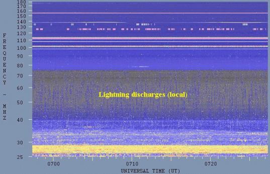
It should be noted that this type of interference is broadband in nature. Individual lightning discharges produce a very short time duration spike. Generally the electrical storm will be within a few tens of kilometres of the radio telescopes. The closer the storm the higher the observed upper frequency limit. This is because the power radiated by a lightning discharge falls off rapidly as a function of frequency, so only bursts that are quite close produce detectable signals at frequencies above 200 MHz.
There is also another aspect about the environment that can modify solar radio signals as received on the Earth's surface. The ionosphere is a plasma and will refract low frequency signals (ie below 100 MHz), sometimes significantly. It is possible for the ionosphere to refract the lower frequency solar signals so that solar bursts may sometimes appear prior to sunrise or after sunset. This requires the solar signal to penetrate the ionosphere in the daytime sector and then be reflected from the ocean (or possibly land surface), and be reflected back down to the receiving station in the night time sector. This requires very unusual ionospheric conditions, possibly a highly ionised sporadic E layer to provide the ionospheric reflection.
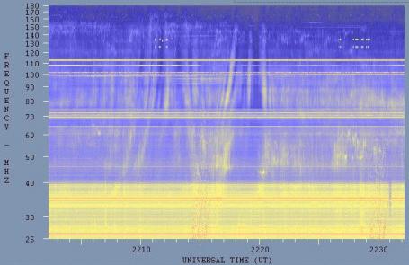
Clumps or inhomogeneities in the ionospheric plasma can also cause modification of a solar signal observed near sunrise or sunset (i.e. when the signal is near grazing incidence to the ionosphere and so travels through a lot of ionospheric plamsa). This can cause an "ionospheric lensing" phenomenon where different frequencies are refracted by different amounts. The result is to introduce structure into what would have been a featureless continuum. I have even seen this phenomenon produce what looked like dozens of type II solar drift bursts. An example of this lensing effect is shown below. Here we can see what appears to be both forward drift (decreasing frequency with time) and reverse drift (increasing frequency with time) bursts. However, they are neither. What we see is produced entirely by ionospheric modification of a patchy solar continuum radio emission. Note that this effect only occurs within about an hour of either sunrise or sunset (with a preference to the latter - probably due to the ionosphere being denser in the latter part of the day).
4.2 Calibration
This section will discuss the calibration of single frequency radiotelescopes or radiometers. Low frequency spectrographs are rarely calibrated in any absolute way, both because of the fundamental difficulty of calibrating a wide range of frequencies, and because environmental effects at low frequencies makes such calibration less than useful.
Because of component variation with environmental parameters and with ageing, radiometer sensitivity changes and needs frequent calibration if it is to provide accurate data.
Accurate data is required to feed computer models and to ensure appropriate customer notification when solar fluxes exceed specified values that have been determined to affect their systems. Data comparisons between two solar radio observatories require both to be well calibrated. And lastly, because the Sun can be viewed from most locations on the Earth, many organisations use the Sun to calibrate their radio equipment (e.g. communications, navigation, radar). This requires that they know accurately the solar radio output at frequent intervals over a wide range of frequencies.
Because the Earth is in an elliptical (although nearly circular orbit) around the Sun, the solar radio flux received by a ground based telescope will vary not only due to intrinsic solar variations but also due to the varying Sun-Earth distance. This distance can change by 3% over the course of a year. To eliminate this variation from our measurements, we standardise our measurements to a distance of one astronomical unit or AU, where
The actual calibration process is one of comparison. We compare the solar signal to a known signal, and compute the solar flux density by a simple ratio. Consider the simplified diagram below where we can switch the input of the radiotelescope receiver between the antenna and a standard signal. These standard signals are normally semiconductor noise sources. They produce a wide band white noise (or Gaussian) signal output with a highly stable output amplitude. It is this stability that makes them a suitable comparison signal source.
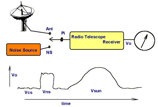
At the input of the radio telescope there is a switch. This could be manually controlled, but most probably we would want it controlled by a computer, so that the calibration can be performed automatically. This switch allows us to select whether the receiver input sees a signal from the antenna or a signal from our standard noise source. Pi is the signal power at the input of the radiotelescope. When the switch is set to "Antenna" then Pi = Pant where Pant is the power that the antenna delivers to the receiver (this will be a minute fraction of a watt). When the switch is set to "Noise Source" then Pi = Pns where Pns is the output power of the noise source.
Now a good radiotelescope has an output voltage Vo that is proportional to the input power (ie the power at the input of the radiotelescope). We can represent this proportionality by the linear equation:
When the antenna is pointed at the Sun and the input switch is set to "Antenna" the input power at the receiver is directly proportional to the solar flux density:
The steps in the process are illustrated by the graph under the above diagram.
First of all we set the input switch to "antenna", and we move the antenna so that it is pointing away from the Sun. This gives us a "cold sky" reading. Because there are no astronomical sources stronger than the Sun above a frequency of 200 MHz, we can take this "cold sky" reading as corresponding to zero solar flux density.
That is, if the output voltage of the telescope has a value of Vcs and we known that S=0, we can easily find the constant b from the above equation:
At this stage we will assume that somehow the noise source has been calibrated, and has an equivalent flux density of Sn. Using this knowledge we can compute the constant "c" as:
Absolute Calibration
The above daily calibration uses a comparison noise source. The obvious question we must now ask is how do we calibrate the "standard" noise source. Noise sources do not and cannot come from the manufacturer with an equivalent solar flux density stamped on them. This is because that value depends uniquely on the radiotelescope itself. In particular, it depends on the effective collecting area of the antenna, and on the losses in the feedline joining the antenna to the receiver.
The effective collecting area of an antenna (Ae) depends on the physical collecting area A (if it is a parabolic dish or similar type of antenna), and on the antenna efficiency. Thus we can write that:
Now for a parabolic dish of diameter d, the area A = π (d/2)2. This can be easily computed. However, the efficiency of such an antenna may vary from about e=0.4 to e=0.8. This efficiency depends of the shape of the parabola, the accuracy of its surface and the characteristics of the antenna feed, which is at the focal point of the parabola. If any of these change with time (for instance a coating of bird poo on the feed), the antenna efficiency will change and with it the need to change the "effective" flux density of the noise source.
We thus need some means of determining the equivalent flux for the noise source. There are several different ways to do this:
1 If we know of another solar radio observatory somewhere else in the world that we believe reports accurate values of solar flux density, we simply change our noise source value until our radiotelescope gives the same value.
2 If we have some way of measuring the actual effective collecting area of the antenna (which is equivalent to determining its efficiency) and also of determining the effective receiver bandwidth B, then we can use a calibrated signal generator to determine the effective flux of our noise source. The physical arrangement is shown in the diagram below:
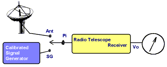
The output of the signal generator can be varied and its output is a known value in watts (actually a very small fraction of a watt). What we do is to adjust the output of the signal generator so that the output of the radiotelescope is exactly equal to the voltage produced when the antenna is pointing to the Sun. This means that the power delivered to the receiver input by the signal generator Psg is identical to the power delivered by the antenna. Thus we can write:
The problem with this method is the determination of the antenna effective collecting area. This normally requires an antenna test range. These are few and far between and are very expensive to set up, and if the antenna is changed in any way on the trip back from the test range to the radio observatory, the measurements become null and void.
3 If the gain of the solar radio telescope can be increased by a sufficient and precisely known amount (and a calibrated signal generator can determine this), then it may be possible to point the antenna at other radio astronomical sources with constant and known flux densities. These can then be used to calibrate the radiotelescope. The problem here is that most other radio astronomical sources have flux densities very much less than the Sun, and below the noise level of most solar radio telescopes, even with the gain turned right up.
4 Although the Sun's radio emissions are constantly changing over many time scales, every 10 to 11 years the Sun returns to a quiescent state. All the sunspots disappear from the surface (ie the photosphere), and all the plage (white) areas vanish from H-alpha images (which allow us to look mainly at the solar chromosphere). At this time there is no slowly varying component (SVC), no transient burst component, and all that is left is the quiet component. If we assume that this quiet component does not vary significantly from one sunspot cycle minimum to the next, we have an easy way of calibrating our telescope - at least once a sunspot cycle.
The graph below gives the best estimate of the solar quiet component from 200 MHz to 15 GHz. The solar flux density for any frequency within this range can be read from the curve below.
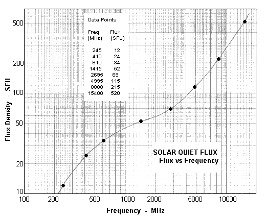
We must just remember that this curve is only a good indication of the absolute solar flux at a time close to sunspot minimum when there are no sunspots visible on the Sun and when an H-alpha image shows no plage.
4.3 Orientation
We must know where the Sun is in the sky, if our radio telescope is to keep track of it as it moves from its rise position in the east and travels to its set position in the west each day.
Now the Sun's apparent movement across the sky is mostly due to the Earth's rotation around its own axis. However, a small component is due to the Earth's revolution around the Sun. Because of this the Earth actually has to rotate not 360o but almost 361o each day to bring the Sun back to the same place in the sky. The Earth's elliptical orbit also means that the Sun's apparent movement across the sky is not exactly constant. Now for most radio telescopes this inconstancy is too small to worry about. Only for large antennas with high enough resolution to image the Sun do we have to worry about this type of second order effect.
There are two general types of mount used in solar radio telescopes. The easiest to drive is the equatorial (sometimes called polar) mount. Because the Sun's motion in declination is small (as it moves back and forth across the equator with the seasons), this type of mount generally only requires to be driven in hour angle (right ascension), and can be driven by a synchronous motor. This is a low cost motor that moves the telescope at a constant rate throughout the day. The declination adjustment can be made manually once a day, or at most a few times each day.
The other type of mount is an elevation-azimuth mount (also called an alt-az mount). This type must be driven in both the azimuth and elevation axes to follow the Sun. And the motors that drive these motions cannot be simple synchronous motors. They must be motors in a feedback loop using encoders that feed back the exact azimuth and elevation angles to a controller that drives the motors. The controller then needs to know the exact elevation and azimuth angles of the Sun at every moment of the day. These values are normally provided by an ephemeris program. The image below indicates the visual display such a program might provide to the observer as well as providing control voltages via a digital to analog converter (DAC) to drive an el-az controller.
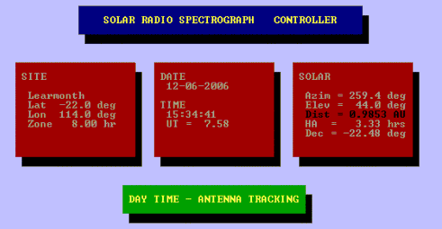
Note that the program calculates both azimuth and elevation coordinates as well as hour angle and declination coordinates. It also provides a value of the Sun-Earth distance in AU (astronomical units), which can be used to correct the solar flux to 1 AU. The only inputs that this program requires are the current date and time (Universal Time is computed from the local time through knowledge of the local time zone - see left box in the display). It is thus essential to have an accurate clock in the observatory. This can be obtained from the internet if the computer has such a connection.
The ephemeris calculations performed by this program are all carried out by a subroutine called SOLPOS whose Quick Basic source code is included below.
SolPos:
  'this code determines various parameters of the sun
  'and uses formulas given at the end of section C of the
  'Astronomical Almanac
  ' The input parameters are the year (yr), month (mn), day (dy) and decimal UT time (UT)
  Day = dy + UT / 24            'UT decimal day
  N = Int(yr + Fix((mn - 9) / 7))               'N is days to J2000.0
  N = -Int(3 * (Int(N / 100) + 1) / 4)
  N = N - Int(7 * (Int((mn + 9) / 12) + yr) / 4)
  N = N - 730516.5 + Day + 367 * yr + Int(275 * mn / 9)
  L = 280.46 + 0.9856474 * N            'mean solar longitude
  L = L - Int(L / 360) * 360            'put in range 0 to 360 deg
  G = (357.528 + 0.9856003 * N) * dr    'mean anomaly
  G = G - Int(G / 2 / pi) * 2 * pi      'put in range 0 to 2*pi
  LA = L + 1.915 * Sin(G) + 0.02 * Sin(2 * G)   'ecliptic longitude
  EP = (23.439 - 0.0000004 * N) * dr    'obliquity of ecliptic
  SD = Sin(EP) * Sin(LA * dr)           ' sin(declination)
  SD = Atn(SD / Sqr(1 - SD * SD))       ' ASIN function
  AL = Atn(Cos(EP) * Tan(LA * dr)) / dr         'right ascension
  If AL < 0 Then AL = AL + 180          'put in correct quadrant
  If LA > 180 Then AL = AL + 180
  If LA > 360 Then AL = AL + 180
  AU = 1.00014 - 0.01671 * Cos(G) - 0.00014 * Cos(2 * G) 'solar distance
  ET = (L - AL) * 4                     'equation of time
  HA = 15 * (UT - 12 + ET / 60 + LO / 15)       'hour angle (deg)
  If HA > 180 Then HA = HA - 360        'put in range -180 to 180 deg
  SE = Sin(LT * dr) * Sin(SD) + Cos(LT * dr) * Cos(SD) * Cos(HA * dr)
  If Abs(SE) = 1 Then                        'singularity
    EL = 90 * Sgn(SE): AZ = 0                'solar elevation and azimuth
  Else
    EL = Atn(SE / Sqr(1 - SE * SE)) / dr     'solar elevation
    CA = (Sin(SD) - Sin(LT * dr) * SE) / Cos(LT * dr) / Sqr(1 - SE * SE)
    If CA = 0 Then                           'CA is cos(azimuth)
      AZ = 90
    Else
      AZ = Atn(Sqr(Abs(1 - CA * CA)) / CA) / dr         'ACOS function
      If AZ < 0 Then AZ = 180 + AZ              'put in right quadrant
    End If
    If HA > 0 Then AZ = 360 - AZ
  End If
  SDd = SD / dr                 'solar declination / degrees
  HAh = HA / 360 * 24           'solar hour angle / hours
Return
The same routine can be used to provide sunrise, sunset and central meridian passage times, which are necessary to know for observing purposes.
4.4 Analysing
Following the task of determining whether a particular increase in radio emission is due to the Sun or to RFI, the next task, assuming the burst is solar in origin, is to classify the type of solar emission you have observed.
Classification for bursts recorded by a single frequency radiometer is quite different to the classifications scheme used for a radiospectrograph.
Radiometer (Single Frequency) Burst Classification
Burst classification for radiometer outputs can only be done in terms of flux density and the time-intensity profile. Such classifications are rather arbitrary and tend to vary from one observatory to another. One simple scheme is shown in the table below.
| Flux Density | Single Peak | Two or More Peaks |
| < 500 SFU | Impulsive burst | Complex burst |
| ≥ 500 SFU | Great burst | Complex great burst |
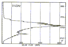
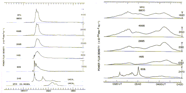
The definition of peaks here is again arbitrary, but generally a significant peak should be separated from another peak by a given time (at least 2 minutes), and should be >20% and >50 SFU above a neighbouring valley. An example of a multi-frequency microwave burst recorded at the Sagamore Hill Solar Radio Observatory is shown below.
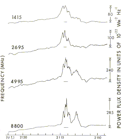
Note that the time scale here runs from right to left. Also note that only the burst on 8800MHz would be regarded as complex. It is the only frequency that has two significant peaks that are just separated by 2 minutes.
There is one type of solar burst that does not fit into the above classification scheme, and that is a solar noise storm. These bursts only occur on frequencies below 1000 MHz, and are most commonly seen in the frequency range from 100 to 300 MHz. This type of burst can have two components. One is a long duration elevation of the solar emission (i.e. a continuum emission), and the other component consists of groups of short duration spikes (each having a narrow bandwidth - only about 2% of the centre frequency - and a duration of seconds). Noise storms may last from hours to days. They almost never exceed 1000 SFU in flux density, with most well below this. And lastly, some bursts are very smooth with no features at all. These gradual rise and fall bursts can be seen in the microwave frequencies. They may last from tens of minutes to an hour or two, and they have very small peak intensities (normally less than 100 SFU).
Bursts around a wavelength of 10 cm (a frequency of 3 GHz) are thought to be more significant than bursts at either lower or higher frequencies, and a special term, a TENFLARE, is used to describe 10cm bursts whose burst amplitude exceeds the background component on this frequency.
Radiospectrograph Burst Classification
Classifications that can be made on the basis of a burst's spectral properties (variations over a significant frequency range as well as with time) are generally more useful.
The CSIRO radiophysics division studied solar radio emissions at metric wavelengths (about 30 to 200 MHz) in the 1950's and devised a spectral classification that is still in use today. They identified five distinct spectral types as follows:
| Spectral Type | Description |
| 1 | This is the spectrograph classification for a noise storm. As for the discrete frequencies, it may be seen with two components - a continuum type emission and a narrow band short duration burst component. Either or both may be present. The radiation is probably a mixture of both plasma and cyclotron radiation. |
| 2 | This is a slow drift burst, and consists of plasma emission from successively higher altitudes in the corona following the passage of a shock wave. This wave may be preceeding the passage of a plasma cloud (CME) through the corona. |
| 3 | This is a fast drift burst, and again is plasma emission following the passage of a high speed (relativistic) stream/beam of electrons through the corona. |
| 4 | This is continuum emission which follows an energetic solar event, such as a large flare or a coronal mass ejection. It is synchrotron emission due to high speed electrons spiralling around the magnetic fields trapped in plasma ejected from or in the corona. |
| 5 | This is continuum emission at low frequencies that follows a type 3. It may be likened to the booming or rolling thunder that occurs after the initial crack of thunder due to a lightning discharge (the initial crack being likened to the type 3). The radiation is probably mostly plasma radiation with some synchrotron component. |
The diagram below indicates the idealised sequence of radio emissions that are often noted to be associated with a large H-alpha flare. However, note that the Sun rarely does the same thing twice, and is continually surprising us. Regard the diagram as indicating a range of phenomena, some of which may occur with any one large flare.
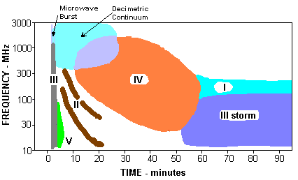
What follows are some examples showing the different types of spectral burst to aid in their recognition.
Type 1 spectral burst
A type 1 spectral burst or solar radio noise storm can be comprised of two different components. One is an elevation of the solar radio emission over a range of frequencies (i.e. an unstructured continuum emission). The other is a series of short narrow band bursts, each independent of any other, at random frequencies within the emission band, and with a bandwidth of about 2%. These will appear as a series of narrow short vertical lines.
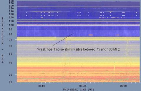
Type 2 spectral burst
A type 2 spectral burst is also referred to as a slow drift burst. It is believed to be due to plasma emission that occurs following the passage of a shock wave through the corona. The shock wave causes a separation of charge centres in the plasma. In restoring the electrical neutrality of the plasma the charges oscillate about each other in damped harmonic motion. The radiation occurs as a result of the acceleration and deceleration that is a consequence of the motion. The frequency of the radiation, also known as the plasma resonance or critical frequency is proportional to the square root of the electron density of the corona from where the emission originates. As this density decreases with altitude in the corona, we can assign an approximate height to each frequency. This allows us to determine the speed at which the shock wave is propagating up through the corona.
The process that creates the type 2 spectral burst generally produces both a fundamental and a second harmonic emission. In most cases both of these emissions are seen on the spectrograph, but on occasion only one may be visible, whether due to creation efficiency at the Sun or due to environmental modification by either the solar or the terrestrial ionsophere (usually refracting the signal so that it is not seen).
Type 3 spectral burst
A type 3 spectral burst is also known as a fast drift burst. These bursts are generally associated with beams of high-speed electrons that shoot up through the corona at speeds that are a substantial fraction of the speed of light. Like type 2 bursts, the radio emission is believed to be plasma radiation that is excited at different levels of the corona by the electron beams as they traverse the region. The speed is so fast that on the image below they appear as near vertical lines, devoid of slope. Higher time resolution is required to show that they do indeed "drift" in frequency.
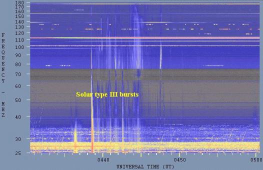
Type 4 spectral burst
This is a continuum radiation (ie emissions simultaneously occurring over a large frequency range) that follows a major solar event (such as a 2B optical flare or an X-class x-ray flare, or in the radio spectrum, after a type 2 burst).
Type 4 emission is often divided into a number of categories (one author lists no less than 16 sub-categories of type 4 burst). The main divisions are threefold: Stationary type 4, Moving type 4, and Flare Continua. Unfortunately a radioheliograph is usually required to distinguish between these.
Type 4 emission will be detectable in a spectrograph display as an increase in brightness (gray-scale) or a different colour (colour map) corresponding to a higher intensity, over a range of frequencies. It normally will not show any structure. The example below is an exception to this rule. It does show structure due to environmental modification (i.e. ionospheric lensing).
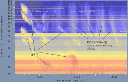
Type 5 spectral burst
A type 5 is not really a separate burst classification, as it refers to short lived continuum radiation at the lower frequencies that follows some type 3 bursts. It is believed to be plasma radiation with a possible admixture of synchrotron emission. It might be likened to the ringing of a bell that follows for some time after the original sound when it is struck, or to the rolling sound of thunder after the initial crack (the crack being analogous to the type 3 and the reverberating noise the following type 5 emission). Thus it might be thought that the type 5 is a ringing oscillation due to reduced damping processes of the plasma radiation, maybe related to magnetic effects.
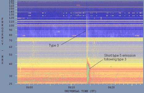
| TYPE | CHARACTERISTICS | DURATION | FREQUENCY RANGE | ASSOCIATED PHENOMENA |
| I | Short, narrow-band bursts. Usually in large numbers with underlying continuum. | Burst ~ 1 second Storm ~ hours to days | 80-200 MHz | Active regions, flares, eruptive prominences |
| II | Slow drifting bursts. Often accompanied by second harmonic. | 5 - 30 minutes | Fundamental ~ 20 - 150 MHz | Flares, proton emission, magnetohydrodyamic shockwaves. |
| III | Fast drifting bursts. Can occur singularly, in groups, or storms. Can be accompanied by second harmonic. | Burst ~ 1 - 3 seconds Group ~ 1 -5 minutes Storm: minutes - hours | 10 kHz - 1 GHz | Active regions, flares |
| IV | Stationary Type IV: Broadband continua with fine structure Moving Type IV: Broadband, slow drifting, smooth continua Flare Continua: Broadband, smooth continua | Hours - days 30 minutes - 2 hours 3 - 45 minutes | 20 - > 1000 MHz 20 - 400 MHz 25 - 200 MHz | Flares, proton emission. Eruptive prominences, magnetohydrodynamic shockwaves, CME. Flares, proton emission. |
| V | Smooth, short lived continua. Follows some type III bursts. Never occurs in isolation. | 1 - 3 minutes | 10 - 200 MHz | Same as type III bursts. |
When analysing solar radio burst events from a spectrograph, as well as the determination of the type of emission, it is usual to report the frequency range over which the emission is observed, the start and end times, and an indication of the emission intensity. Because many solar radiospectrographs are not calibrated (at least in an absolute sense), and because the environment (particularly the ionosphere) can easily make a mockery of calibrations on the lower frequency (due to attenuation, refraction, scattering and interference), it is usual to employ a limited quantised scale of intensity. This may have only three values (low, medium and high), sometimes described as minor, significant and major. Such a scale is of course relative and subjective.
When the radiation is plasma radiation and the burst shows a drift with time, it is possible to compute the speed at which the shock wave responsible for the plasma emission is moving through the corona. To do so we use the equations presented in section 2.6. In practical form these become a single equation relating frequency to height:
There are two practical points that we need to consider in doing this. A slow drift burst will normally show both a fundamental and a harmonic component. If you use the second harmonic to measure the plasma frequencies, you must first divide these frequencies by 2 to get the required fundamental frequencies to substitute in the above equation.
The second point is that because the leading edge of a burst is often quite ragged, two measurements may not provide a very accurate speed estimate. It is usual to take several measurements and use these in a multiple regression least squares analysis to get a more accurate result. This is usually done by computer.
Shock speed calculations are normally only done for slow drift bursts (type 2 spectral classification). Fast drift (type 3) bursts travel at a substantial fraction of the speed of light and are due to beams of relativistic electrons. These lighter particles are normally not significant for space weather purposes. Accurate measurement of their speeds, if wanted, requires a high resolution timebase, which can only be obtained by sweeping the frequency spectrum more rapidly, with a resultant tradeoff of signal to noise ratio.
Slow drift bursts typically have shock speeds between 200 and 2000 km/sec. Note that solar escape velocity is just under 620 km/sec.
Castelli-U spectral event
There is one type of microwave spectral event that we have not so far mentioned. This requires either a spectrograph that covers the range from 200 to at least 10 GHz, or a number of fixed frequency radiometers that cover the same range with no more than octave spacings between them (an octave is a frequency range of 2:1 - for example from 500 to 1000 MHz or 2 to 4 GHz).
This type of spectral burst was investigated by John Castelli of the USAF Research Laboratories in the late 1960's. It gets its name from the U shape that it displays on a intensity versus frequency plot. It was once initially thought that the presence of a U-shaped spectrum was indicative of a solar proton flare, the most damaging event that occurs on the Sun (with respect to equipment and humans in space). These events are sometimes known as Solar Cosmic Ray events.
Further analysis showed that a Castelli-U is simply the typical spectral form of microwave bursts for most large solar events. However, the presence of a C-U spectrum together with type 2 and type 4 metrewave bursts are usually a good indication that processes in the Sun have accelerated protons to relativistic speeds.
The requirements for a Castelli-U are four-fold:
(1) the burst must show a peak of >1000 SFU on frequencies < 1GHz
(2) a near simultaneous (within 2 minutes) peak >1000SFU on high microwave freqs
(3) a dip in mid-microwave frequencies - to produce the U shape
(4) the integrated flux of the burst on 8800 MHz must exceed 100,000 SFU-secs
The plot below shows a Castelli-U spectral burst.
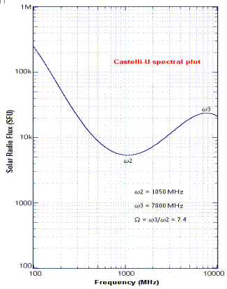
The graph below show the proton flare that commenced within 20 minutes of a Castelli-U/type2/type4 complex of radio spectral bursts.
4.5 Reporting
To save anyone but the original analyst from having to wade through the raw data time and time again, it is usual (as well as useful) for the analyst to report all significant radio emissions in tabular (or coded) form. The immediate report is useful to space weather forecast centres for nowcasting and predictive purposes. It also allows lists to be compiled of such solar radio emissions that can be used for scientific studies. Such lists are usually compiled, kept and distributed from world data centres.
Only significant parameters should be reported for each solar radio event. Suggested parameters for single frequency radiometers and spectrographs are given below.
Radiometer Solar Burst Reports
Spectrograph Solar Burst Reports
4.6 Housekeeping
As with many other jobs, observing and immediate analysis are not the only tasks that must be carried out in conducting continuous radio patrol of the Sun.
Quality control is very important. This means rechecking data to ensure that reports previously issued were accurate and that no solar activity has been missed. If possible it is preferable that a person other than the originator of the analysis and reports should do the checking.
Archiving data is also another important housekeeping function. Raw data should be copied from hard drives onto CD or other format storage media and sent to one or more of the various World Data Centres around the world. It is useful to keep at least a subset of this data on site for training purposes, research reports and public relations (and maybe even to ensure data survival through major natural and man-made catastrophes).
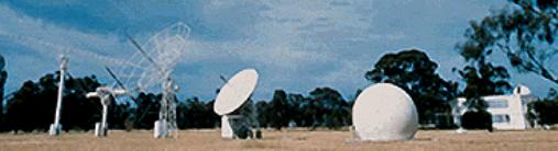
5 LEARNING MORE
So, where to from here? Unfortunately there are very few books written specifically on solar radio astronomy. These are listed below:
Mukul R Kundu, "Solar Radio Astronomy", Interscience[Wiley] (New York, 1965)
Alex G Smith, "Radio Exploration of the Sun", Van Nostrand (Princeton, 1967)
Albrecht Kruger, "Introduction to Solar Radio Astronomy and Radio Physics", Reidel, (Dordrecht, 1979)
MR Kundu and Tomas R Gergely (Editors), "Radio Physics of the Sun", Symposium at College Park, Maryland, Aug 7-10, 1979, Reidel, (Dordrecht, 1980)
AO Benz and P Zlobec (Editors), "Solar Radio Storms", Proceedings of the 4th CESRA Workshop on "Solar Noise Storms", Trieste (1982)
DJ McLean & NR Labrum (Editors), "Solar Radio Physics", Cambridge University Press (Cambridge, 1985) ISBN 0 521 25409 4
While some of these may be useful for people involved in research into solar radio emissions, the only two that are readable for those interested in solar radio patrol for space weather purposes are the first two. The small book by Smith is eminently readable, and you should find the first few chapters of "Solar Radio Astronomy" by Kundu quite helpful as well. Both of these texts however were written about 40 years ago. "Solar Radio Physics" written by McLean and Labrum is a more recent summary of what CSIRO learnt about the subject over 40 years, before the Radiophysics group changed direction (and the text was written so that this knowledge would not be lost). There is certainly some very useful information to be gained from this text, but a lot of it is quite technical and mathematical. The Cambridge font and layout unfortunately does not make for easy reading.
The two most significant journals for articles on solar radio physics are
Solar Physics
and
Journal of Geophysical Research (JGR) - blue (series A).
In particular you might check out articles in the last 10 years by Bill Erickson and his wife Hilary Cane. They argue that there is a subclass of type 3 emission, which they term 3L (L for occurring later and at lower frequencies than the initial type 3 emission that occurs preceding a type 2/4 complex). They present data to show that 3L emission is very often associated with proton events.
Over the last 15 years a controversy has developed over the nature of the shock wave that produces the type 2 burst that we observe at metric wavelengths. The CME "camp" (ie those group of people who believe that CME's "cause" everything) have stated that they believe that type II's are only the result of blast waves produced by flares (which produce the Moreton/Ramsay waves we see in H-alpha images), and are thus only solar surface or low atmospheric phenomenon, with nothing to do with CME's, and are thus useless in predicting travel times for CME's to Earth. Interplanetary observations however, have shown that a least one group of type 2's are associated with CME propagation. It is very possible that we need to sub-classify type 2 emissions into at least 2 groups.
There is some useful tutorial material on the web. One of these is a series of lectures on solar radio physics by Dale Gary of the New Jersey Institute of Technology.
And finally there is nothing like experience accumulated from continuous and long term observation of the Sun.
 Australian Space Academy