DEFINITION
The designation 'coronal mass ejection' or CME is used in two ways. As an active principle it refers to the eruptive release from the solar corona (the Sun's outer atmosphere) of a large cloud of plasma containing several billion tons of material in which is embedded solar magnetic fields. As an entity it also refers to the plasma cloud or magnetic cloud itself.
GENERATION
CMEs occur from regions of the Sun in which the magnetic field is closed, but which suffer an extremely energetic disruption. The ejection velocity appears to vary from a very few hundred kilometres per second up to around 1500 km/sec. Those CMEs travelling at less than the solar wind speed are accelerated toward that speed, and those with a higher velocity are decelerated toward the solar wind speed as they travel through the interplanetary medium.
OBSERVATION
|
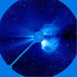
CMEs are most spectacularly observed by a white light coronagraph located outside the Earth's atmosphere. Such observations from Skylab in the early 1970's were the first in which the phenomenon was recognised. SOLWIND (P78-1) and SOLAR MAXIMUM MISSION (SMM) were routinely used at the end of the 1970's and early 1980's for routine observation and study of CMEs. However the SOHO spacecraft with its large scale coronagraph (LASCO) was the one that brought CME's to a wide audience. (See image to the left). Spacecraft in the interplanetary medium with plasma measuring instruments on board (eg ACE) can measure the passage of a CME as it moves past. CMEs detected in this way are sometimes referred to as Interplanetary CMEs or ICMEs. |
OCCURRENCE
The frequency of CMEs has been observed to vary from once every few days to several times a day. As with solar flares, the occurrence rate varies from sunspot minimum to sunspot maximum, although it does not follow the sunspot number exactly. Large CMEs are usually associated with large flares but the correlation drops for smaller CMEs and smaller flares.
A very approximate relationship between daily CME occurrence and the smoothed sunspot number is given by:
The only real conclusion that such a relationship implies is that both CMEs and sunspots are different manifestations of global solar magnetic activity.
MORPHOLOGY
The observed form of CMEs is currently very much dependent on our observational biases. Because past white light coronagraphs have only observed CMEs from near the Earth, CMEs travelling toward the Earth appear to be quite different from those travelling at right angles to our line of sight. We thus distinguish limb CMEs and halo CMEs. The latter appear to surround or nearly surround the occulted solar disc in the coronagraph, and are those CMEs that are heading towards (or away from) the Earth. Some but not all CMEs appear to have a hollow or plasma deficient core region.
EFFECTS
The most prominent effect of a CME is when it passes by the Earth and creates a geomagnetic storm. CME plasma makes its way into the Earth's magnetosphere. Plasma particles spiral and precess around the Earth's magnetic field in such a way as to diminish the internal component of the field (this is referred to as the storm main phase depression). Particles also precipitate to lower altitudes, particularly around the polar regions and are removed from circulation upon collision with neutral atmosphere molecules. All this motion produces oscillations in the magnetic field as seen on ground and orbiting magnetometers.
For a CME to produce a geomagnetic storm it is important that the magnetic field it carries points in a southerly direction. Only with this orientation will the plasma be able to couple into the Earth's magnetosphere. Northerly directed fields cut off plasma entry into the near Earth environment.
Another less well known effect of a CME is the scintillation of point radio sources. If a radio telescope is observing a source of small angular extent, such as a quasar, and a CME passes the line of sight between the radio telescope and the radio 'star', the amplitude and phase of the signal will show irregular variation or scintillation, much as the Earth's atmosphere causes visible twinkling of stars.
PRECURSORS AND PREDICTIONS
Predicting the occurence of CMEs is one of the main goals of space weather research.
The research group led by Dick Canfield at Montana University has noted that a sigmoidal shape observed in X-ray images of the Sun is almost invariably associated with generation of CMEs, although the latency can be quite variable (from hours to days).
Hilary Cane and associates have indicated that what they have classified as a type 3L radio burst is strongly associated with CME release. The L stands for low frequency (below 50 MHz) and long duration (in comparison with other type 3 radio emission).
Some but not all type II radio bursts are associated with CMEs. The association becomes more likely when a type IV is also present.
Long duration X-ray increases are almost always accompanied by coronal mass ejections. Such events are also reflected as gradual rise and fall radio bursts in the mid-microwave spectrum.
We should also note that because there is an almost 100% correlation between large flares and large/fast CMEs, all the conventional indications that have been used to predict flares (sunspot group configuration and photospheric magnetic configuration) are also going to be applicable to CME prediction.
A SIMPLE MODEL
A simple model of a CME assumes rough spherical symmetry of the plasma cloud.
As the plasma cloud moves out from the Sun it expands so that its
volume:
Some typical values for a CME:
     Solar distance             Diameter       Magnetic Field
      r(million km)	      L(million km)     B(nanoTesla)

        10 {15 solar radii}       1.0              1000
        20		          1.6               250
        30                        2.0               111
        40		          2.5                63
        50		          2.9                40
        60 {Mercury orbit}        3.2                28
        70		          3.6	             20
        80		          3.9	             16
        90		          4.2	             12
       100		          4.6	             10
       110 {Venus orbit}          4.9                 8
       120		          5.1	              7
       130		          5.4	              6
       140		          5.7	              5
       150 {Earth orbit}          6.0	              4
SOLAR-TERRESTRIAL TRAVEL TIME
The following table lists the travel time for a CME to reach the Earth (assuming of course that it is travelling in the right direction). Three different models are shown. The linear model assumes that the CME is travelling along an interplanetary field line curving out from the Sun at an angle of about 45 degrees.
	Speed	Linear	Wang	Gopals
	(km/s)	(hrs)   (hrs)   (hrs)

	  200	 295	 133	 109
	  300    196      98     104
          400    147      81      99
          500    118      70      92
          600     98      63      85
          700     84      58      77
          800     74      54      69
          900     65      51      62
         1000     59      49      54
         1100     54      47      48
         1200     49      46      42
         1300     45      44      37
         1400     42      43      34
         1500     39      42      33
         1600     37      41      33
Note that the input for these models (CME speed at the Sun) is rarely available from optical observations, and often the plane of the sky velocity will be used. This will result in a large scatter of the predicted time compared to the actual travel time because such a velocity includes the expansion of the CME as well as any true velocity component.
Australian Space Academy
 Home
Home