A STUDY ON THE EFFECTS OF BINARY MOTION ON THE DETECTION OF RADIO PULSARS
by Owen Giersch
Note: The material presented here was submitted as an honours thesis at Curtin University in 2002
ABSTRACT
The detectability of binary pulsars was determined by modelling the signal from binary pulsars with differing orbital parameters. These signals are then Fourier transformed to obtain the power spectrum. These spectra can then be studied in order to determine the likelihood of detection. The modelling for over 40,000 orbits was successfully achieved and their detectabilities determined. These results are displayed as a series of contour plots.
CONTENTS
1.0 INTRODUCTION
Radio pulsars are usually detected by analysing the power spectrum of the signals received by a radio telescope. For isolated pulsars this spectrum should contain a sharp peak. However, for a binary pulsar the Doppler shift resulting from the pulsarís orbital motion will distort the signals and the power spectrum will be broadened and reduced in amplitude. This selection effect may account in part for the relative scarcity of binary pulsars as compared with binary stars. Current theory also suggests that the rarity of binary pulsars may be a function of these systemsí evolution.
A series of binary pulsars with different orbital configurations will be computer modelled. The signals from these systems will be analysed to determine the power spectrum. The frequency and power will then be plotted against orbital elements such as eccentricity and inclination. A measure of detectability will also be plotted against orbital elements.
By analysing these power spectra, the detectability of binary pulsars can be determined. Hence, the effectiveness of current detection techniques can be evaluated.
Only radio pulsars will be considered in this analysis and only a limited range of systems will be able to be examined. However the software will be designed to model any realistic binary pulsar system.
2.0 OVERVIEW OF PULSARS
Pulsars are thought to be rapidly spinning neutron stars that have an intense magnetic field. The magnetic field is inferred from the radiation beaming presumably from the magnetic poles of the neutron star. If the magnetic poles are at some angle to the geographic poles, the radiation beam will rotate and may be detected as it sweeps across the Earth.
2.1 Structure of a Neutron Star
A neutron star is thought to have a structure as shown below:
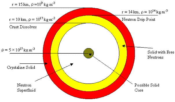
Figure 2.1.1: Structure of a Neutron Star (Lyne & Graham-Smith, 1990)
The crust is a rigid and strong crystalline lattice composed mainly of iron nuclei. At higher densities, electrons penetrate the nuclei and combine with protons to form nuclei with high numbers of neutrons (eg Kr-118). Up to a density of about
4x10¹⁴ kg m-3 there are no free neutrons. Past this density (referred to as the neutron drip point) massive nuclei become unstable and are embedded in a neutron fluid. The core consists of a neutron fluid with small numbers of electrons and protons. There is the possibility of a solid core past densities of 3x10¹⁷ kg m-3 (Lyne & Graham-Smith, 1990) 19).
The theoretical allowable masses for neutron stars lie between 0.2 and 2.0 solar masses (MS). A smaller mass has insufficient gravity to hold the star together whereas a larger mass will collapse further to form a black hole. The moment of inertia is approximately constant for all neutron stars because a larger mass is more condensed (Lyne and Graham-Smith, 1990). The diameter of a neutron star of mass 1.4 MS has a radius of 20 to 30 km and has a central density of 1017 kg m-3(Lyne and Graham-Smith, 1990). The uncertainty in size arises because of uncertainties in the equation of state.
The measured masses of neutron stars fall in a narrower range than the theoretical masses. Most neutron stars seem to have a mass lying between 1.3 and 1.5 MS (Thorsett and Chakrabarty 1999). Below is a diagram showing the measured masses of 21 pulsars.
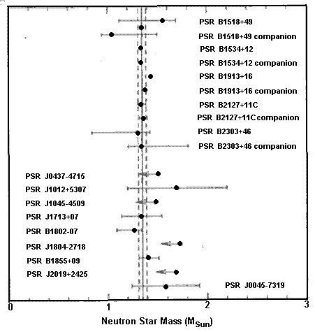
Figure 2.1.2: Measured masses of 19 neutron stars. The error bars are at 68% confidence. Five double neutron stars are shown at the top. Open circles indicate that the average mass is better known than the individual masses. The middle eight have white dwarf companions and the last has a main sequence companion (Thorsett and Chakrabarty, 1999).
It is important to note that the masses can usually only be determined if the pulsar is in a binary system (Thorsett and Chakrabarty, 1999).
2.2 The Magnetic Field of Neutron Stars
Polar field strengths of 108 Tesla can occur in young pulsars. In old pulsars this may drop to 106 T. For millisecond pulsars it may be as low as 104 T. These fields have little effect on the structure of the star except for a slight modification of the crystalline surface (Lyne and Graham-Smith, 1990). Outside the star the induced electrostatic forces are some 12 orders of magnitude greater than the gravitational forces. Thus the electrostatic force dominates all physical processes around the star (Lyne & Graham-Smith, 1990).
To understand the origins of the magnetic field, it is necessary to understand the physical processes that occur within the pulsar; specifically those within the neutron fluid. The neutron fluid is broken up into a series of quantised vortices due to the allowable quantum states within the fluid (Sauls, 1988). There are approximately 2x10⁹ vortices per square metre (Lyne & Graham-Smith, 1990). The individual neutrons are paired in a way similar to superconducting electrons: ie they form Cooper pairs. Within the neutron fluid there are a small number of protons that form a superconductor. These protons are linked with the crust by means of a magnetic field and co-rotate with the crust without forming vortices (Sauls, 1988). This proton superconductor is thought to be responsible for the magnetic field.
The magnetic dipole of a pulsar is thought to be substantially misaligned with the axis of rotation of the pulsar. This produces an electromagnetic wave at the rotational frequency. A local electric field is induced by the magnetic field and is of overwhelming influence to a distance
 . . . (2.2.1)
where rc is the distance where a co-rotating particle with period P would have a velocity of the speed of light.
This defines the dimensions of the velocity of light cylinder. It is within this cylinder, in an ionised ďmagnetosphereĒ of high energy plasma, that the radiation beam originates. The magnetic field links the neutron fluid to the rotation of the star by means of the small number of electrons and protons in the fluid (Lyne & Graham-Smith, 1990).
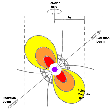
Figure 2.2.1: Diagram of the radiation beam of a pulsar. rc defines the velocity of light cylinder (Lyne & Graham-Smith, 1990).
2.3 Observed Pulsar Pulse Shapes
Individual pulses from the same pulsar can vary greatly. Therefore a convenient measure of the pulse shape is the integrated pulse profile. A series of about one hundred pulses are added to produce an average pulse profile. The integrated pulse does not vary greatly. That is two different sets of pulses from the same pulsar will have a similar integrated pulse profile (Graham-Smith, 1988).
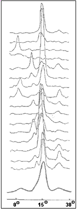
Figure 2.3.1: A series of pulses are summed to give the integrated pulse profile (Graham-Smith: 1988)
The integrated pulse profiles of 31 pulsars are shown below.
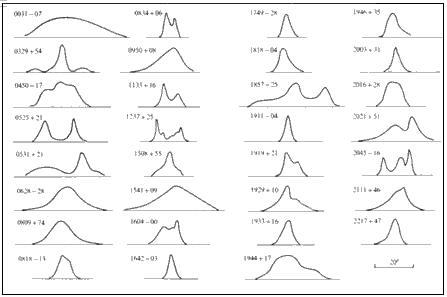
Figure 2.3.2: The integrated pulse profiles for 31 pulsars (Graham-Smith, 1988)
The integrated pulse profiles usually have a small number of components to them and occupy 2% to 10% of the period (Graham-Smith, 1988). Note that the pulse profile can vary greatly with the radio frequency at which the pulse is observed, but usually the pulse broadens at low frequencies (less than 1 GHz). This is largely due to differences in spectral index between components (Lyne and Graham-Smith, 1990).
Some pulsars have a large interpulse. This is thought to be due to a nearly orthogonal magnetic field so that both poles sweep past the earth (Lyne and Graham-Smith, 1990).
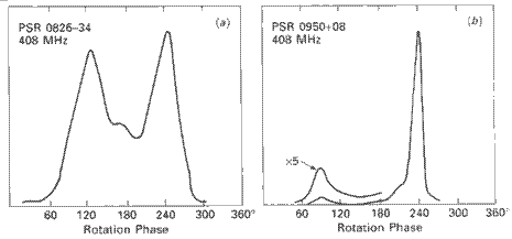
Figure 2.3.3: Two pulse profiles showing an interpulse (Lyne and Graham-Smith, 1990)
For the purposes of this investigation all of the pulses will be assumed to be identical, that is the individual pulse profiles will assumed to be the same as the integrated pulse profile. Using Fourier analysis it will be possible to reconstruct an entire pulse profile from its harmonics.
2.4 Evolution of Pulsars
Most of the discovered pulsars reside in the Milky Way. The only extra-galactic pulsars discovered are in the Magellenic Clouds. Most pulsars are young galactic objects. Their distribution is similar to young massive stars and supernovae. There are estimated to be (3.5 +/- 1.5)x105 active pulsars in the Milky Way. Most of these are not luminous enough to detect (Lyne & Graham-Smith, 1990).
The lifetime of a pulsar is of the order of ten million years. This is small when compared with the lifetime of the galaxy. Hence a constant population of pulsars can be assumed. It is estimated that the pulsar birthrate is between one every 30 to 120 years (Lyne & Graham-Smith, 1990).
The ages of a pulsar can be estimated by making some assumptions about the slowdown rate of the pulsar. Magnetic braking will slow down the pulsar. This happens because some of the energy of rotation of the magnetic dipole is radiated away. A simple power law is used to model the slowdown.
 . . . (2.4.1)
where Ω is the frequency of rotation, k is a constant and n is referred to as the braking index.
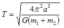
Equation (2.4.1) can be used to derive the characteristic age. Lyne and Graham-Smith (1990) have a full derivation. The expression for the characteristic age, Τ is:
 . . . (2.4.2)
where P is the period of rotation.
The parameter n has a value of 3 for a rotating magnetic dipole, giving:
 . . . (2.4.3)
As an example, the Crab Pulsar supernova event was observed by Oriental astronomers 900 years ago but shows a characteristic age of 1250 years. This difference is accounted for by an outflow of particles from the pulsar adding an additional torque (Lyne & Graham-Smith, 1990).
The birth of pulsars is thought to occur mainly in supernovae. Supernovae fall into two categories: type I and type II. Type I supernovae spectra contain many lines from heavy elements. The type II spectra are primarily from hydrogen. Type II supernovae originate from more massive stars that have an extensive envelope of gas that obscure the underlying radiation from the outer parts of the star (Lyne & Graham-Smith, 1990).
The energy source for a supernova explosion is the release of gravitational energy as the star collapses catastrophically. This results from a failure of the central energy supply. The main sequence of stars maintain hydrostatic equilibrium between thermal pressure and gravitation while hydrogen is converted into helium. For a star of mass 1 MS the fuel supply lasts for about 1010 years. A star of mass 10 MS lasts for about 106 years (Lyne & Graham-Smith, 1990).
When the hydrogen is exhausted, helium burning follows in the core, the temperature of which has reached 2x10⁸ K, while the outer envelope has cooled and expanded. The star is now a red giant. The coreís evolution proceeds independently of the outer envelope (Lyne & Graham-Smith, 1990).
Different stages of nuclear burning can proceed in different layers until iron is produced in the core. Less energy is available at each stage and hence each stage lasts for a shorter period of time. Gravitational collapse follows, but the type of collapse depends on the mass of the core. From 1.9 MS to 2.5 MS, the core will collapse to form a neutron star, releasing about 1 MS in the process. Less massive cores may explode due to carbon burning occurring catastrophically in a carbon flash. In more massive stars the core will collapse into a neutron star or black hole soon after carbon burning has started. A black hole will result if the core has a mass greater than 2.5 MS (Lyne & Graham-Smith, 1990).
Collapse to form a neutron star via a type II supernova occurs for stars with a total mass between 8 and 15 MS. A type I supernova will occur for masses of 2 to 8 MS leaving no neutron star. For masses above 15 MS the star will become a type II supernova, but the core may become a black hole or photodisintegrate (Lyne & Graham-Smith, 1990).
[Photodisintegration is the process by which nuclei are blown apart due to the high energy of photons produced in the core of massive stars.]
3.0 BINARY PULSARS
3.1 Evolution of Binary Pulsars
The first mechanism is by supernova. Consider two stars of mass 25 MS and 8 MS, as shown in figure 3.1.1 (i). The heavier primary star evolves more quickly reaching the giant stage before the companion has changed. The companion then fills its Roche lobe (the point where the gravitational forces in the system balance) (ii). The mass is then transferred to the smaller star and their masses practically interchange, leaving only a helium core for the primary (iii). This is called a Wolf-Rayet binary. This core then evolves rapidly and explodes leaving a white dwarf or neutron star (iv). The secondary now evolves more rapidly filling its Roche lobe and transferring mass back to the primary (v). When this happens a large amount of energy is released producing an x-ray binary. The secondary can then go supernova, leaving a neutron star (Lyne & Graham-Smith, 1990).
The mass lost in this system may disrupt the binary. Disruption is only avoided if more than half of the system mass is ejected in the explosion (van den Heuvel, 1988). Type I supernovae are expected to remain bound while type II will disrupt the binary system leaving two high velocity stars (Lyne & Graham-Smith, 1990).
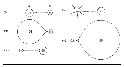
Figure 3.1.1: Stages in the evolution of a binary pulsar (Lyne & Graham-Smith, 1990).
Supernova explosions are probably not frequent enough to account for the pulsar birthrate. Another way a neutron star may form is if a white dwarf can accrete material from a companion. This is thought to occur in close binary systems with a star of mass less than 5 MS. Mass transfer will occur from the primary when it is approaching the helium burning phase. The whole envelope is transferred to the companion leaving a core to evolve on its own. If this leads to a collapse to a white dwarf, there may be accretion in the reverse direction as the companion evolves. This may lead to the collapse of the white dwarf to a neutron star leaving a millisecond pulsar (Lyne & Graham-Smith, 1990).
Note that both of the evolution scenarios described above do not lead to a binary pulsar with certainty. In the first case, disruption of the binary is likely. In the second case, the companion may evaporate. This may be occurring in PSR 1957+20 (A. S. Fruchter et. al, 1988).
Final possible evolutionary paths may occur in globular clusters. An isolated neutron star can capture a non-degenerate star to form a close binary system (Johnston and Kulkarni, 1991). The maximum orbital radius of these systems is approximately 5 RS which will give an orbital period of less than one day. The less massive the secondary the closer the orbit and shorter the period (Johnston and Kulkarni, 1991).
An alternative method is that a white dwarf may capture a star and subsequently accrete material from it. If the white dwarf achieves a sufficient mass it may form a neutron star (Johnston and Kulkarni, 1991).
In either case a close bound system will result, making detection more difficult. Also there are difficulties in these types of formation. In the first case, models for globular cluster formation suggest that the rate of neutron star formation is too low. In the second case, highly variable stars should be visible, but as yet they remain undetected (Johnston and Kulkarni, 1991).
3.2 Evolution of Millisecond Pulsars
Millisecond pulsars are all thought to form in binary systems. Orbital angular momentum is transferred from the binary orbit to rotational energy of the pulsar. Hence they are effectively spun-up. The characteristic ages for millisecond pulsars are of the order of 109years (Lyne & Graham-Smith, 1990). In addition most unbound millisecond pulsars have high proper motions, suggesting that they may have been ejected from a binary system.
3.3 Orbital Mechanics
To determine the time of arrival of a signal from a binary pulsar, it is necessary to consider the orbit of the pulsar. A mostly Newtonian approach is taken in this description. The only relativistic effects that will be considered are the orbital period decay, time dilation due to the pulsarís velocity and the gravitational redshift. Thus only orbits where the velocities are small compared with the speed of light will be considered. The derivation of the expressions is not given here. For a complete derivation see chapter 6 of Spherical Astronomy by Green (1985).
Consider the orbit of a pulsar as shown below:
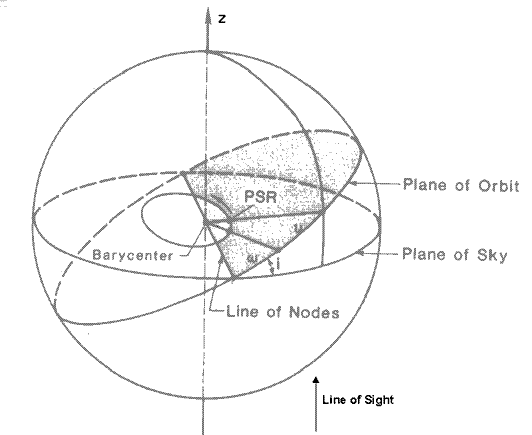
Figure 3.3.1: A binary pulsar orbit (Backer and Helling, 1986).
Here ι is the inclination of the orbit and ranges from 0 to π/2, and ν is the true anomaly. m1 will be the mass of the pulsar (the primary) and m2 is the mass of the companion* . ω is the argument of periastron (position of closest approach) and is defined from the line of nodes. The line of nodes is where the great circle that the pulsarís orbit lies in intersects with the celestial sphere. This point, Ω, is defined from the x-axis.
* [ This differs from the usual definition in binary star systems. Usually the largest mass star is referred to as the primary. For binary pulsars, the pulsar is referred to as the primary regardless of its mass. ]
The position of the pulsar at any time t is required. A series of relatively simple steps can be followed in order to obtain the position.
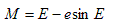
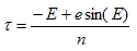
The first step is to calculate the mean anomaly, M, for the pulsar.
 . . . (3.3.1)
where Τ is the time of periastron and n is the mean motion given by:
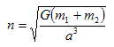 . . . (3.3.2)
where a is the semi-major axis of the pulsarís orbit and G is the gravitational constant.
Next, the eccentric anomaly, E, is found by solving the following expression:
 . . . (3.3.3)
where e is the eccentricity of the pulsar orbit.
Note that E will be 0 at periastron. E is found by using the Newton-Raphson method.
Now r, the distance to the binary barycentre, can be found:
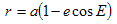 . . . (3.3.4)
Also, the true anomaly can be found:
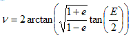 . . . (3.3.5)
The only other parameter which is required is z, the position of the pulsar along the line of sight:
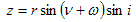 . . . (3.3.6)
Other parameters which will be of use are T, the period of the orbit, and Tb, the lifetime of the system due to gravitational wave energy losses.
 . . . (3.3.7)
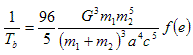 . . . (3.3.8)
(Backer and Hellings, 1986), where
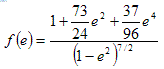 . . . (3.3.9)
Finally the time of periastron, Τ, will need to be found. It is assumed that t=0 at the line of nodes. Therefore Τ can be found using the following method:
At t = 0, ν= -ω and E is found using
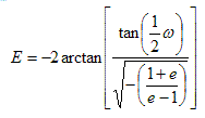 . . . (3.3.10)
 . . . (3.3.11)
3.4 Timing Equation
To derive the timing equation several factors need to be considered. However, it will be assumed that the signal has been corrected to the solar system barycentre (TDB) and that it has also been corrected for dispersion. Dispersion is caused by the signal interacting with electrons in the interstellar media (Backer, 1988).
This leaves three other factors to consider: the Doppler effect, time dilation due to variations in the pulsars velocity in its elliptical orbit and the gravitational redshift from the companion.
The timing equation for a binary pulsar is:
 . . . (3.4.1)
where
 . . . (3.4.2)
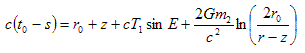
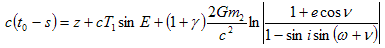
t0 is the observed time of arrival
s is the time of emission
r0 is the distance to the barycentre of the binary pulsar
(Green, 1988)
Here, r0 will be constant and can be dropped from the equation without affecting the analysis to follow.
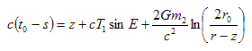 . . . (3.4.3)
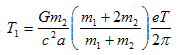
The third term can be replaced by a more convenient term
 . . . (3.4.4)
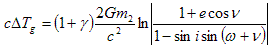
where ΔTg is the gravitational time delay and γ=1 (This assumes that general relativity is correct). (Backer and Hellings, 1986). Substituting (3.4.4) for the last term in (3.4.3) gives:
 . . . (3.4.5)
The first term on the right hand side of equation (3.4.5) is the first order Doppler shift due to the pulsarís motion. The second term accounts for the time dilation effect due to variations in velocity along the pulsarís orbit. The third term accounts for the gravitational red shift due to the influence of the companion. Overall the right hand side of equation (3.4.5) will result in a phase shift of a pulse depending on the position of the pulsar in its orbit. Since the true signal can be decomposed into Fourier series components, the pulsar signalís first harmonic can be modelled as:
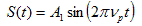 . . . (3.4.6)
where A1 is the amplitude of the first harmonic, νp is the frequency of the signal and S is the current value of the wave. Then at the solar system barycentre the following phase-shifted signal will be observed:
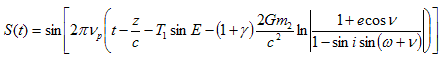 . . . (3.4.7)
where A1 can be rejected without loss of generality.
4.0 FOURIER ANALYSIS
4.1 The Continuous Fourier Transform
Any cyclical function can be represented as infinite sum of sine and cosine terms. However, it is often more convenient to represent a Fourier Transform in its complex exponential form.
Suppose there is some function S(t). Itís Fourier Transform is given by:
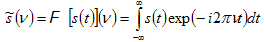 . . . (4.1.1)
where
s is some function of t
ν is the frequency
F is the Fourier transform operator
š is the Fourier transformed signal
(Gonzalez and Wintz, 1987)
The inverse Fourier transform is given by:
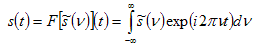 . . . (4.1.2)
(Gonzalez and Wintz, 1987)
The Fourier transform gives the harmonics present in any function. Note that there are some functions whose Fourier series diverges. These functions are considered to be pathological (DeVries, 1994).
The Fourier transform produces a complex spectrum. It is often more useful to convert this to a real spectrum (Fourier Spectrum) especially when plotting the spectrum. The Fourier spectrum is given by  . Furthermore the Power spectrum is given by:
 . . . (4.1.3)
[ Most of the above expressions come from Gonzalez and Wintz but the notation has been changed to conform with Jouteux et al. (2002) ]
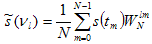
4.2 The Discrete Fourier Transform
Experimental data are rarely continuous. Thus the above approach must be modified in order to obtain the Fourier spectrum. This is done by replacing the integral with a sum.
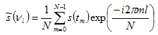 . . . (4.2.1)
where m is the sample number, l is the bin number in the Fourier spectrum, ν is the frequency and N is the number of uniformly spaced samples (Gonzalez and Wintz, 1987). Similarly, the inverse Fourier transform is:
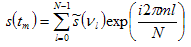 . . . (4.2.2)
(Gonzalez and Wintz, 1987)
The frequency and time are related by:
 . . . (4.2.3)
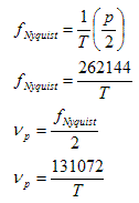
Care must be taken when using equation (4.2.1). The frequencies (N/2)Δν up to ((N/2)-1)Δν are actually negative frequencies from Ė(N/2)Δν to Δν. The highest frequency which can be obtained is referred to as the Nyquist frequency and is given by fNyquist = (N/2)Δν. (DeVries, 1994).
Thus it is possible to extract frequency information about a signal from its time data. Of course the faster the sampling rate the better the frequency resolution obtained.
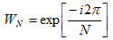
4.3 The Fast Fourier Transform (FFT)
The drawback with the Fourier Transform is that it is computationally expensive. The Fourier transform requires N2 complex calculations. Thus a faster method is required for transforming a large number of points. This is done by using the Fast Fourier Transform (FFT).
The FFT requires that the data be split into two sets. An analysis is then performed on each set separately. This derivation for the FFT can be found with more detail in Gonzalez and Wintz (1987).
 . . . (4.3.1)
where
 . . . (4.3.2)
Also N = 2M where M is a positive integer.
Now equation (4.3.1) can be written as:
 . . . (4.3.3)
Equation (4.3.3) is equivalent to:
 . . . (4.3.4)
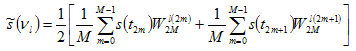
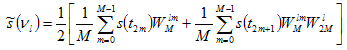
Equation (4.3.4) can be written in two parts as follows:
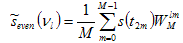 . . . (4.3.5)
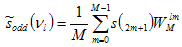 . . . (4.3.6)
The complete Fourier Transform is obtained as follows:
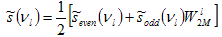 . . . (4.3.7)
and
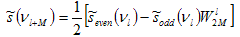 . . . (4.3.8)
Each of the even and odd data sets are themselves discrete sets and these can be broken into even and odd sets. This process can be repeated until each set holds only one value (DeVries, 1994).
The main advantage of this method is that it only takes Nlog2N calculations rather than N2 calculations. However N must equal 2k where k is a positive integer.
There are generally two solutions to the constraint on N. One is to add zeros to the data either at the beginning or end (or both) so that N=2k. The other is to use an algorithm which splits the data up into more groups, for example N=3n. With the former approach, corrections may need to be made if phase is important (Bracewell, 2000).
4.4 Useful Properties of the Fourier Transform
The main theorem of use is the Similarity Theorem. Suppose a signal s(t) has a Fourier Spectrum š(ν) . If the time series is compressed by some factor a, the resulting Fourier Spectrum will be given by.
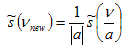 . . . (4.4.1)
All harmonics in the spectrum will be effected equally (Bracewell, 2000).
For some types of analysis, the phase of the signal may be important. The phase is given by:
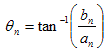 . . . (4.4.2)
where bn and an are the imaginary and real components for the nth frequency (Pain, 1993).
The Power theorem can be used to check that no significant rounding errors have occurred. This is also called the energy theorem and is written as:
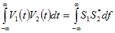 . . . (4.4.3)
where S1 and S2 are the Fourier transforms of V1 and V2 (Bracewell, 2000). The asterisk indicates the complex conjugate.
For discrete data equation (4.4.3) can be written as:
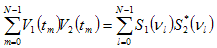 . . . (4.4.4)
If V=V1=V2 then equation (4.4.3) can be written as:
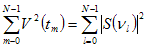 . . . (4.4.5)
The right hand side of equation (4.4.5) is simply the power as described in section 4.1. The left hand side is simply an alternative expression for the power. Thus this relationship can be used to ensure there are no problems with rounding errors in the Fourier analysis.
5.0 THE BINARY PULSAR MODEL
5.1 Assumptions and Parameters
In order to model the binary pulsar systems it is necessary to clarify exactly what assumptions are made. In this model, a mostly Newtonian approach is taken. Thus only orbits which are non-relativistic can be modelled. Relativity is used to calculate the variation in the emission times due to the changing velocity of the pulsar in its orbit. This is caused by the elliptical path of the pulsar. The gravitational red shift is also included even though this effect is expected to be small.
The current value of the signal s, can be summarised as follows:
 . . . (5.1.1)
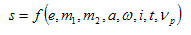
All of the other orbital parameters can be calculated from these seven. Of these parameters, one of e, ω or ι will be an independent variable, x. The (s, t) data set for each value of x will undergo a Fourier transform. This data will be used in order to obtain a graphical representation of the power spectrum and detectabilty for a given pulsar system. Thus any one system may have many different plots. Note that Ω, the position of the line of nodes, has no effect on the observed signal as this only affects the orientation of the pulsarís orbit perpendicular to the line of sight.
The parameters e, m1, m2, ι and a are restricted to certain values due to either the physical constraints on the system or the constraints on the model.
The actual masses of neutron stars are expected to vary from about 1.3 MS to 1.5 MS. For this model a pulsar mass of 1.4 MS will be used. The mass of the companion m2 can have a much wider range. In general the companion is either a white dwarf (typical mass < 0.4 MS) or a neutron star (typical mass 1.3 MS to 1.5 MS) (Thorsett and Chakrabarty, 1999). Two binary pulsars have been discovered with main sequence companions. These are both type B stars. The main sequence companion with the best mass estimate (J0045-7319) has a mass of 10 +/- 1 MS (Thorsett and Chakrabarty, 1999).
Most binary pulsars have a nearly circular orbit. The majority of the remainder have highly eccentric orbits. The largest eccentricity is 0.8699310 for the pulsar
PSR J1302-6350 (ATNF Pulsar Catalogue).
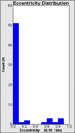
Figure 5.1.1: Histogram showing distribution of eccentricities for 62 binary pulsars. 51 have circular or nearly circular orbits and 8 have highly eccentric orbits.
The semi-major axis, a, of a binary pulsar can also vary greatly. The value of a will largely depend upon the orbital period which is of interest. The shortest period binary pulsar yet discovered is JRA dec R and has a period of 95.3 minutes (Jouteux et al. 2002). If this has a white dwarf companion, then the expected value for a would be around 3.8x10⁻³ AU. If it has a neutron star companion then a would be around 4.5x10⁻³ AU. The semi-major axis will be restricted simply because the maximum period that will be examined is 48 hours. For any given system, both of the masses and the period will be known, producing an upper limit on the value for a.
The orbit of the pulsar can have any inclination. However, an edge on orbit (ι=π/2) will show the greatest Doppler shifted signal (both by its motion and gravity by the companion). A face on orbit (ι=0) will show no Doppler shift. Also, the most probable orbit is edge on (Thorsett and Chakrabarty, 1999).
In modelling these orbits it is hoped that ω will have little or no effect on the power spectrum and that the inclination will produce a steady, continuous and predictable change. If this is the case, then the amount of modelling can be reduced.
Finally any system modelled will be checked to ensure that it has a sufficient lifetime and does not decay by gravitational radiation too rapidly.
5.2 Simulating Pulses
A pulsarís signal is simulated by a sine wave of frequency νp. This will represent the fundamental frequency of the pulsarís signal. This is then corrected to account for the orbit of the pulsar. The observed signal will be given by equation (3.4.7) The results can be generated for higher harmonics of the pulsar signal.
5.3 Coding
The program was written in Fortran 90. The general algorithms will be described below. For the complete pseudo-code see Appendix 1.
Firstly the user creates a file which contains the list of the parameters for each system to be modelled. See Appendix 3 for the format of this file. The pulsar modelling program then reads this file and begins processing each system.
The frequency of the pulsar signal is found by:
 . . . (5.3.1)
where T is the orbital period of the pulsar.
This frequency is chosen because it will lie in the middle of the spectrum. This minimises the spread of the signal exceeding the Nyquist frequency.
Calculations for the orbits now begin. e and ω are both calculated. By the end of each systems modelling there will be ωmax+1 orbits for each eccentricity giving a total of (ωmax+1)(emax+1) spectra where ωmax and emax are supplied in the input file (see Appendix 3).
The program increments e and ω systematically. For each e and ω, an orbit is modelled using the equations described in section 3.3 and the observed pulsar signal is generated using the equations described in sections 3.3 and 3.4. This signal is Fourier transformed in order to obtain the power spectrum for the particular orbit. A measure of detectabilty is then calculated by dividing the highest peak in the spectrum by the total power in the spectrum.
The program outputs four files for each system analysed. The data file contains the power spectrum for each orbit modelled. The detection file holds the detection measure for each orbit. The log file contains the parameters of the system and data for each orbit. If for some reason an orbit could not be computed, the log file contains the reason why. The axis file contains axis titles and ranges for use in plotting the data. Appendix 2 contains the exact format for each of the output files.
Each data file is then read into a plotting program which generates the plots.
There are several important issues which must be taken into account when generating this data.
Firstly, the log term in the timing equation can be problematic for certain orbits. This term will be undefined when ν+ω = π/2 and i = π/2. In order to overcome this problem the orbit is examined to ensure that the above condition does not occur. If it does a small shift is placed on the starting time.
The second consideration is the amount of data collected. There are 524288 points in the signal. There will be half that number in the power spectrum (the negative frequencies are ignored as they have the same amplitude as the positive frequencies). Each one of these is double precision (4 bytes per number) giving 1 megabyte per signal. It is expected that each file will have 10201 signals which would give a total amount of data of over 10 gigabytes per system. Thus a data reduction algorithm is implemented which removes values which are close to zero (less than 1x10-11) that lie outside the area of interest in the power spectrum.
The third consideration is precision. All of the terms in the timing equation are accurate to order c-2 or better. Numerically this equates to 1.11x10⁻¹⁷. This is better than machine precision (1x10-15). Furthermore, the Newton-Raphson method has a precision of the square root of machine precision (3.16x10⁻⁸ in this case). Hence the effective precision of the equations is far greater than the precision that the computer can generate.
5.4 Parallel Processing
The program is run a parallel machine, thus the option exists to write the program so that it can utilise more than one CPU.
Most parallel computers implement a standard called Message Passing Interface (MPI). Simply put, this standard enables the CPUís to communicate with each other by passing messages to each other. A message is simply some piece of data. It can be text, integers, real numbers, complex numbers or some other data type (including user defined data types).
A common way of using this type of processing is for breaking up loops and getting each processor to do only one piece of the loop.
For the pulsar modelling program each processor is given a set of orbits. Each processor calculates the spectra for these orbits and the data is passed back to one CPU in order to write the data to file.
The computer used for this project was the Compaq SC40 located at IVEC. This system comprises four ES40 AlphaServers each with four 667 MHz CPUís. Each ES40 node has 4 Gigabytes of RAM and 36 to 108 Gigabytes of disk space. This machine is rated at 20 Gigaflops (2x10¹⁰ floating point operations).
6.0 RESULTS
6.1 Program Testing
The first step in testing the various algorithms was to confirm that the orbits were being calculated correctly. Figure 6.1.1 shows a sample set of orbits. Only the z position is shown even though the true anomaly is of importance. This figure demonstrates that the orbits are being calculated correctly.
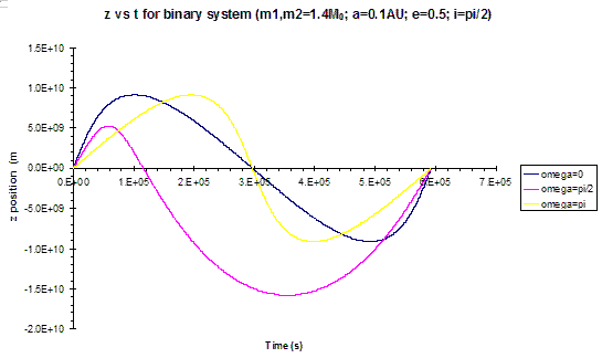
Figure 6.1.1: z vs t for a sample binary system.
The next step was to ensure that the signal and its corresponding phase shift was being calculated correctly. Figure 6.1.2a shows a sample spectrum for which the inclination was 0 (face on). Figure 6.1.2b shows the same orbit except for i=π/2 (edge on). Figure 6.1.3 shows a both of these plots on a log scale. As can be seen the peaks for the edge on orbit are much lower than for the face on orbit. A contour plot was generated to show this effect (Figure 6.1.4). As inclination increases, the height of the peaks decreases thus making these orbits less detectable. Thus most of the systems modelled have an edge on orbit, since this is the worst case for detection. It is understood that as inclination decreases, the detectability increases for all cases.
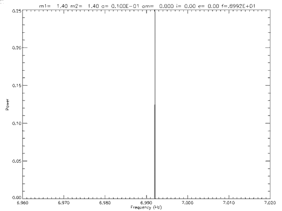
Figure 6.1.2a: Power spectrum for a face on (i=pi/2) orbit.
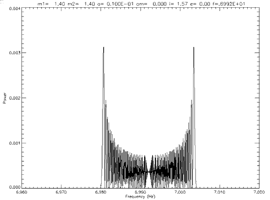
Figure 6.1.2b: Power spectrum for an edge on orbit.
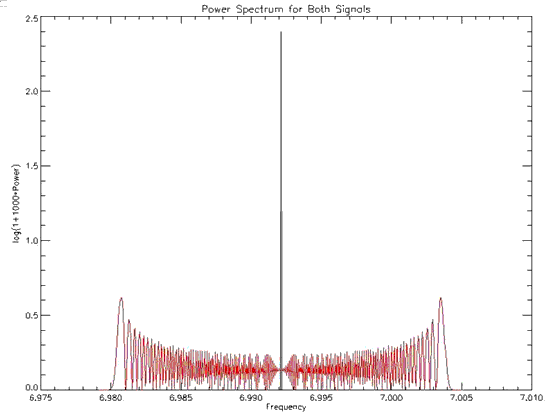
Figure 6.1.3: Logarithmic plot of the power spectrum for a face on and edge on orbit.
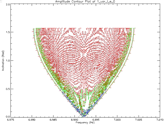
Figure 6.1.4: Contour Plot of a system with the following parameters: m1=1.4MS, m2=1.4MS, a=0.01 AU, ω=0, e=0. Inclination was varied. For this plot, the blue contours are the highest power, green the next highest and red the lowest power.
The phase shift for these systems was calculated without the addition of the gravitational red shift. The velocity of the pulsar for these orbits was too slow to show any time dilation effect.
A preliminary analysis of the effect of argument of periastron on the pulsarís power spectrum was performed. Several spectra of eccentric orbits are shown below.
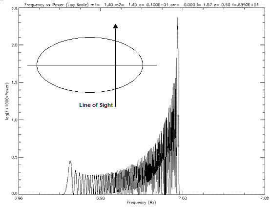
Figure 6.1.5a: Power spectra for a binary pulsar of e=0.5 and ω=0. The inset shows the orientation of the orbit. The pulsar will be moving in an anti-clockwise direction.
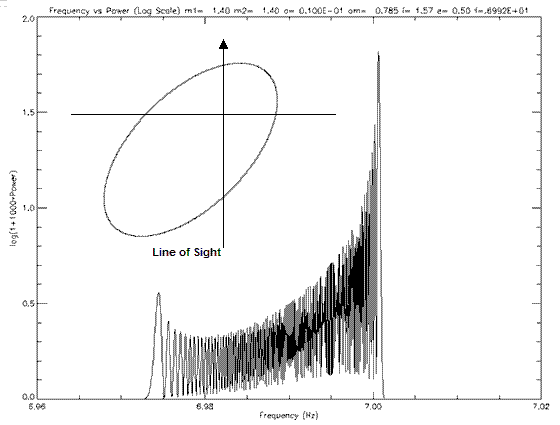
Figure 6.1.5b: Power spectra for a binary pulsar of e=0.5 and ω=π/4. The inset shows the orientation of the orbit. The pulsar will be moving in an anti-clockwise direction.
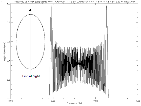
Figure 6.1.5c: Power spectra for a binary pulsar of e=0.5 and ω=π/2. The inset shows the orientation of the orbit. The pulsar will be moving in an anti-clockwise direction.
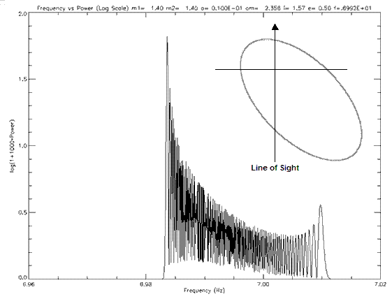
Figure 6.1.5d: Power spectra for a binary pulsar of e=0.5 and ω=3π/4. The inset shows the orientation of the orbit. The pulsar will be moving in an anti-clockwise direction.
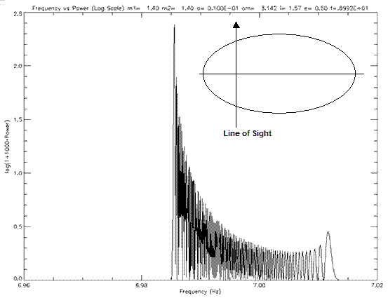
Figure 6.1.5e: Power spectra for a binary pulsar of e=0.5 and ω=π. The inset shows the orientation of the orbit. The pulsar will be moving in an anti-clockwise direction.
These plots show that argument of periastron does greatly effect the power spectrum of a binary pulsar. The shape of the power spectra varies with argument of periastron and the peak heights also vary. Observation along the semi-minor axis will produce larger peaks in the power spectra, thus being the best case for detection. A greater analysis was performed by varying eccentricity and argument of periastron and determining these orbits detectability.
6.2 Discussion
The programs were tested and data was generated on a Pentium 266 computer to ensure that there were no catastrophic errors in the code. Once the code was debugged the program was up-loaded onto the SC40 computer at the IVEC laboratories and tested in order to ensure that there were no compiler differences. Once all problems were removed from the code, several systems were modelled in order to determine their detectability. A graphical representation of detectability was generated using contour plots.
It took approximately 2.7 seconds in order for the program to model a single orbit, generate the pulsar signal, calculate the power spectrum and determine its detectability. Since each of the systems modelled contained 10201 orbits, the maximum time required to generate a complete set of data is approximately 7.65 hours on a single CPU. As more CPUís are used the time decreases proportionately. For most of the data collected, four CPUís were used giving a total time to generate the data for one plot of 1.9 hours. This is a maximum time, for a variety of reasons some orbits were unable to be calculated, thus program execution usually took less time. It was usually not possible to use more than four CPUís due to the requirements of other userís.
All of the subsequent plots were generated using commercial plotting software. The detection plots did not require any data reduction . The frequency - power plots did require data reduction simply because the plots appeared to be cluttered.
As stated previously, the detection efficiency of a pulsar was found simply by dividing the highest peak in the power spectrum by the total power. This was the way detection was measured up until 1990. The system for a given detection plot is given in the title for each plot. It should be noted that the gravitational red shift was not included for the following results.
Figure 6.2.1 shows a typical detection efficiency plot for a neutron-neutron star system with a semi-major axis of 0.1 AU. It is clearly obvious that the shape and orientation of the pulsarís orbit affect detection. It can be seen that if the line of sight is along either the semi-minor axis (ω=0), detection is improved. Conversely, if the line of sight is along the semi major axis (ω=π), detection is poor. This is due to the differences in the pulsarís velocity for these cases. Furthermore, eccentric orbits along the semi minor axis seem easier to detect. Figure 6.2.2 is a log plot of the same data in order to show additional detail.
Figure 6.2.3 is a similar system except with a=0.01 AU. As can be seen from the contour values, most orbits in this system are less detectable than those in Figure 6.2.1. However this system becomes more detectable at high eccentricities. Note that Figure 6.2.3 has no values for an eccentricity greater than 0.9. This is the point where the orbits became too relativistic in order to model using the Newtonian equations.
Two other detection plots can are shown in figures 6.2.4 and 6.2.5. Both of these have a=0.01 AU but have a companion mass of 0.3 MS (white dwarf) and 10.0 MS (type B star). The more massive of these systems is in general less detectable.
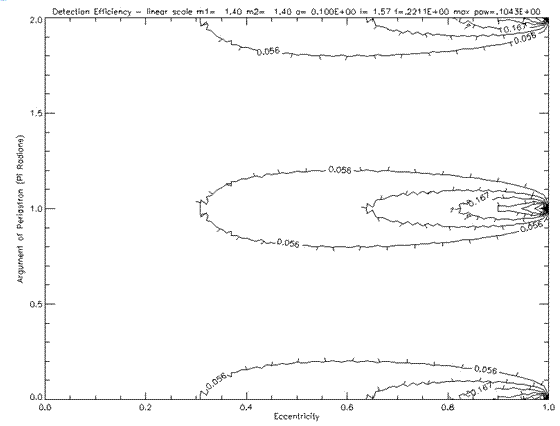
Figure 6.2.1: Contour plot of detection efficiency for a neutron Ė neutron star system with a=0.1 AU.
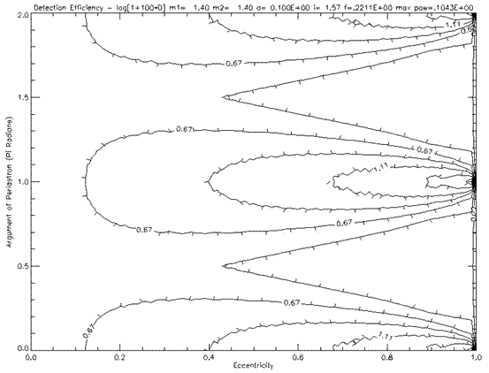
Figure 6.2.2: Log contour plot of detection efficiency for a neutron Ė neutron star system with a=0.01 AU
A fifth systemís modelling was attempted. This was a neutron-neutron star system with a=0.001 AU. This system was too relativistic to obtain any data, even for circular orbits.
From these results some general patterns can be observed. Firstly, that argument of periastron and eccentricity effect detection of binary pulsars significantly. The best case for detection is observation along the semi-minor axis of the ellipse, and the orbit being highly elliptical. All of the systems modelled seem to have a similar general shape for the detection plots. As expected, the orbital period affects detection. The shorter the period of a pulsarís orbit, the harder it is to detect due to the Doppler effect.
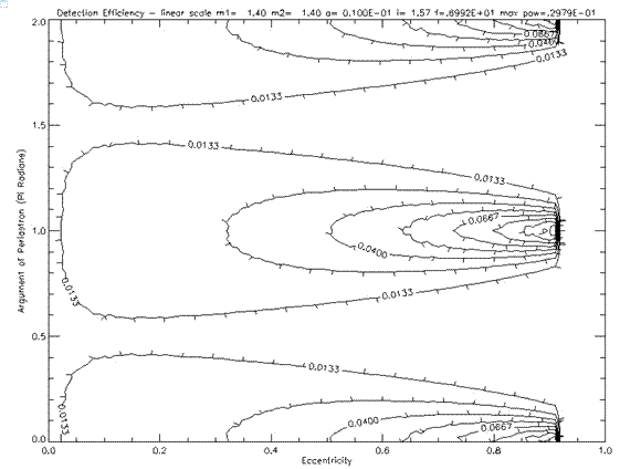
Figure 6.2.3: Contour plot of detection efficiency for a neutron Ė neutron star system with a=0.01 AU.
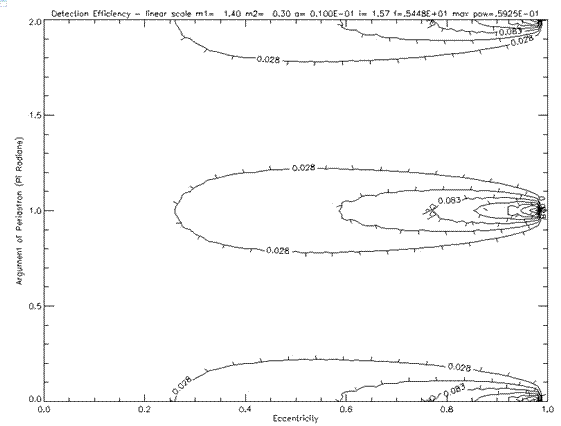
Figure 6.2.4: Contour plot of detection efficiency for a neutron Ė white dwarf star system with a=0.01 AU.
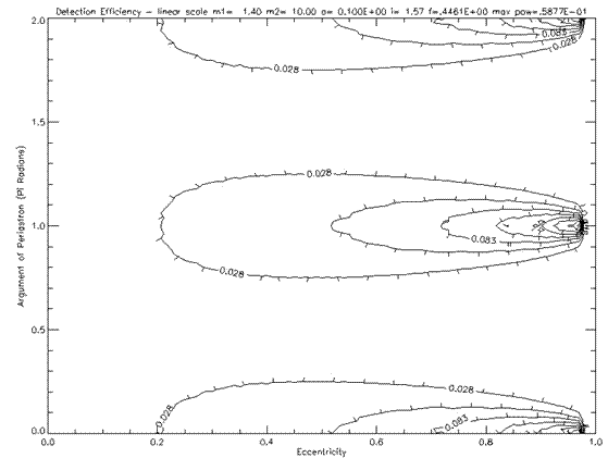
Figure 6.2.5: Contour plot of detection efficiency for a neutron Ė type B star system with a=0.1 AU.
7.0 FUTURE WORK
At this stage, only the power spectra has been analysed, and a rather crude measure of detectabilty has been used. This was largely due to the computational requirements of other detection algorithms, especially the Partial Coherence Recovery Technique (Jouteux et al. 2002, 539). However, it seems little work as been done in investigating the phase of the pulsar signals. It is hoped that there is some systematic variation in the phase which would be able to be extracted from noise. This of course would mean that any information about power would be lost. The pulsarís signal phase is expected to rotate an extra 2? per orbit. The calculations done to this date do not show this, and it is yet to be determined whether the phase is being calculated correctly.
ACKNOWLEDGEMENTS
The author would like to acknowledge the help of his supervisors in producing this work:
- Dr Jamie Biggs
- Dr Mario Zadnik
APPENDICES
The appendices contain information on the program code used in the simulations described above. They may be found in the file BINPULSA. If anyone is interested in the FORTRAN 90 code used to implement the simulations they should send a request to the author, Owen Giersch, at <odg@spaceacademy.net.au>.
REFERENCES
Lyne, A. G. and Graham-Smith, F., 1990, Pulsar Astronomy, Cambridge University Press, Cambridge, New York
Green, Robin M., 1985, Spherical Astronomy, Cambridge University Press, Cambridge
Gonzalez, Rafael C. and Wintz, Paul, 1987, Digital Image Processing, 2nd Edition, Addison-Wesley Publishing Company, Massachusetts
Alpar, M. A., 1988, ĎInside Neutron Starsí, Timing Neutron Stars, 431
Graham-Smith, F., 1988, ĎThe Radio Emission From Pulsarsí, Timing Neutron Stars, 133
van den Heuvel, E. P. J., 1988, ĎStellar Evolution and the Formation of Neutron Stars in Binary Systemsí, Timing Neutron Stars, 523
Backer, D. C. and Hellings, R. W., 1986, ĎPulsar Timing and General Relativityí, Ann. Rev. Astron. Astrophys., 24, 537
Haugan, Mark, P., 1985, ĎPost-Newtonian Arrival-Time Analysis for a Pulsar in a Binary Systemí, The Astrophysical Journal, 296, 1
Pain, H. J., 1993, The Physics of Vibrations and Waves, 4th Edition, John Wiley & Sons, Chichester
Bracewell, Ronald N., 2000, The Fourier Transform and its Applications, 3rd Edition, McGraw Hill, Boston
Thorsett, S. E. and Chakrabarty, D., 1999, ĎNeutron Star Mass Measurementsí, The Astrophysical Journal, 512, 288
Johnston, Helen M. and Kulkarni, Shrinivas R., 1991, ĎOn the Detectability of Pulsars in Close Binary Systemsí, The Astrophysical Journal, 368, 504
Jouteux, S., Ramachandran, R., Stappers, B. W., Jonker, P.G. and van der Klis, M., 2002, ĎSearching for Pulsars in Close Circular Binary Systemsí, Astronomy and Astrophysics, 384, 532
DeVries, Paul L., 1994, A First Course in Computational Physics, John Wily and Sons Inc., New York
 Australian Space Academy