SOLAR RADIO INTERFERENCE TO SATELLITE DOWNLINKS
 |
John A Kennewell
[ An earlier version of this material was presented as a paper at
ICAP 89, the Sixth International Conference on Antennas and
Propagation, held at Warwick University UK, 1989. ]
|
1 OVERVIEW
No long distance communication system is free from environmental
disturbances of one kind or another. High frequency communication
depends on the vagaries of the ionosphere. VHF and UHF
transionospheric systems experience problems due to rapid changes
in the ionospheric electron density. SHF and EHF links are subject
to tropospheric attenuation, and all space-Earth links are subject
to potential disruption when the Sun enters the beam of the downlink
receiving antenna. This latter well known phenomenon (sometimes
referred to as a "sun-outage") is commonly associated with wideband
downlinks from geosynchronous satellites, but at times of high
solar activity any electromagnetic receiving system pointed near
the Sun may experience disruptive effects.
This note reviews the nature of solar radio emissions and provides
appropriate conversion algorithms between solar radio astronomical
terminology and useful communication parameters. Algorithms for the
computation of the duration and severity of solar disturbances are
provided, with graphical examples showing the effect of various
parameters.
2 ELECTROMAGNETIC EMISSIONS FROM THE SUN
2.1 General
The Sun, by nature of its high temperature, is a wideband radio
emitter. Its size also makes it a source to be reckoned with
when low noise electromagnetic receiving systems are pointed
toward it. Futhermore, the variability of its output makes it
difficult to predict its exact effect on a given system.
It is convenient to divide the solar radio emission into three
separate components. These are referred to as the background
component, the slowly varying component and the burst component.
Each of these can be identified with separate sources on the Sun.
Figure 1 is a photograph of the Sun taken in the light of the
hydrogen-alpha spectral line. This shows the solar chromosphere,
the "inner atmosphere" of the Sun. It is from this region, together
with the lower part of the corona (the Sun's "outer atmosphere"),
that radio emissions in the 1 to 20 GHz range originate. The
featureless areas of the solar disc (or the regions above them) may
be regarded as the source of the background component. The light
white areas, termed plage, are several thousand degrees hotter than
the background areas, and these are the primary source of the slowly
varying component. Plage areas and sunspot groups occur in the same
regions of the Sun, both phenomena being due to the emergence of
large magnetic fields from lower depths. The intensely bright
area is a solar flare, an explosive process whereby magnetic energy
is converted into large quantities (up to 1025 Joule) of
electromagnetic energy. It is these events that are responsible for
the burst component.
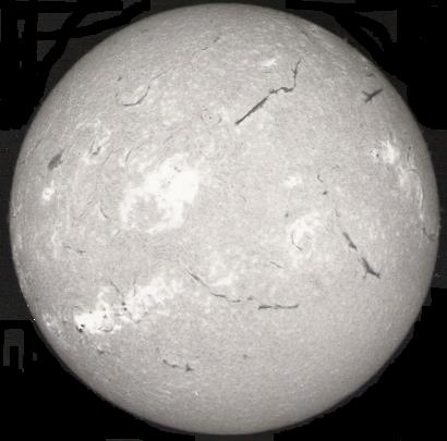
Figure 1 - The solar chromosphere - the source of solar microwave emission
[ Learmonth Solar Observatory image ]
When measuring the whole disc radio emission of the Sun, radio
astronomers typically use the Solar Flux Unit or SFU which equals
10-22 W m-2 Hz-1. Figure 2 shows the typical range of flux
densities appropriate to each of the three components.
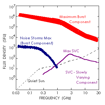
Figure 2 - Solar Radio Spectra
2.2 The Background Component
The background or quiet component of the solar emission is by definition
the component that remains when all variable components have been
eliminated. It is thus a constant at a given frequency and it is
estimated to an accuracy of 10% within the range 1 to 20 GHz by the
following second order polynomial:
Sq = 26.4 + 12.4 f + 1.11 f 2 (1 < f(GHz) < 20) ... eq 1
At the higher frequencies within this range the emission is uniformly
distributed across an area only a few percent larger than the visible
disc of the Sun. However, at the lower end of the range, the radio Sun
is rather larger than the optical Sun, and a limb brightening effect
is noticeable (figure 3). This is in contrast to limb darkening
that occurs at visible wavelengths. The variation in radio output
across the solar disc is only significant when the antenna beamwidth
is less than the angle subtended by the Sun (approximately 0.5
degrees).
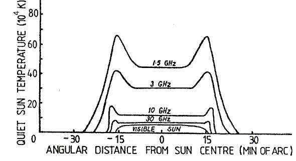
Figure 3 - Spatial Variation of Solar Microwave
Emission ( after Kundu [ref 4] )
2.3 The Slowly Varying Component
The slowly varying component shows a variation on two quite different
time scales. The first, of approximately 27 to 28 days, is the rotation
period of the Sun at mid-latitudes (the equatorial rotation rate is
substantially greater than the polar rate) where plage is most
predominant. This component is due to the uneven longitudinal
distribution of plage. As an area of intense and extensive plage
rotates onto the visible disc (as seen from Earth) this component will
increase. A small plage area may grow and decay within a day. A
large area may persist for several solar rotations. This process will
also produce random fluctuations with component periods less than a
rotation. The second component varies in accompaniment with the
sunspot cycle in an approximately 11 year cycle (figure 4).
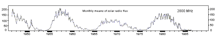
Figure 4 - The smoothed variation of the slowly varying component
with time. Individual values within a month can exceed 300 SFU
(Algonquin Radio Observatory, after SGD [ref 5] ).
The slowly varying component is essentially produced by specific
regions on the Sun, and thus shows a significant spatial variation
over the disc. Examples several days apart are shown in figure 5.
Again, this spatial variation is only important when the antenna
beamwidth is a fraction of the angle subtended by the Sun.
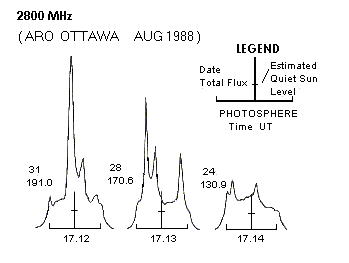
Figure 5 - Spatial variation of slowly varying component
The slowly varying component has a maximum value at a frequency of
around 3GHz and falls off at higher and lower frequencies. At 1 Ghz
and 30 Ghz the value has fallen to about 25% of the value at the peak
frequency. The flux density at any frequency f(GHz) can be estimated
to within 10% by the following expression:
Sv (SFU) = [ 0.64 ( F10 - 70 ) f 0.4 ] / [ 1 + 1.56 ( ln ( f / 2.9 ) )2 ] ... eq 2
where F10 is the current value of the solar radio emission at a
wavelength of 10.7cm (2800 MHz). This value is measured and made
available from the Penticton Radio Observatory in Canada. It is also
available on a daily basis from various space environmental services,
and is broadcast on some standard frequency and time services
(eg WWV, WWVH). The function ln( ) is the natural logarithm.
Over one sunspot cycle S may range from 0 to above 250 SFU. Note that
F10 is in fact the value of Sq + Sv at 2.8 GHz.
2.4 The Burst Component
This component is a transient emission associated with explosive energy
releases in the solar chromosphere and corona. At metre wavelengths
it may increase the total solar output by six orders of magnitude,
the increase lasting anywhere from seconds to hours. The frequency
at which these bursts occur varies throughout the sunspot cycle, with
very low probabilities when F10 is at a minimum, to several times a
day at times of activity maximum. The intensity of the bursts also
shows an ill defined average correlation with burst frequency,
although large isolated bursts have been known to occur irrespective
of other general solar activity. In the frequency range of 1 to 20
GHz, the average maximum flux density for the largest bursts typically
varies from 100,000 to 10,000 SFU respectively. An exception to this
was noted in December 2006 when two L-band bursts to around one million
SFU were recorded.
No empirical expression is possible for the burst component Sb. Some
space weather agencies may attempt probability forecasts for interested
parties. A moderate duration high intensity burst is shown in figure 6.
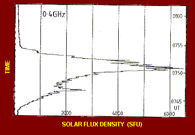
Figure 6 - Moderate intensity solar radio burst
[ Learmonth Solar Observatory ]
2.5 Summary
The total solar radio emission is specified by S = Sq + Sv + Sb.
However, in most applications Sb is taken as zero. A non-zero burst
component is usually readily identifiable by the presence of a large
and fluctuating noise level.
The nature of the solar signal is identical to the thermal (Gaussian)
noise generated in receiver circuitry. The power collected by a
receiving antenna is given by:
P = S Ae (W Hz-1) ... eq 3
where Ae is the effective collecting area of the antenna.
This expression is appropriate where the total solar emission is being
collected - that is, an antenna beamwidth greater than the solar
diameter with the Sun totally within the beam. For large antennas
on the higher frequencies, the beamwidth may be less than the solar
disc (figure 7). In these cases the antenna essentially assumes the
temperature of that part of the Sun to which it points. Under the
assumption of a uniform brightness, this temperature is given in terms
of the integrated flux density S by:
Tsun = S λ2 / ( 2 k Ωs ) ... eq 4
where λ is the wavelength, k=1.38x10⁻²³ J K-1 is Boltzmann's constant
and Ωs = 6.8x10⁻⁵ steradians is the mean solid angle subtended by
the Sun. At sunspot minimum, Tsun ~10,000K at 20 GHz. The assumption
of uniform surface temperature is valid at sunspot minimum, but
becomes increasingly non-valid, especially around 3 GHz and lower
frequencies, as F10 rises above 100 SFU. It is more valid at
frequencies of 10 GHz and above.
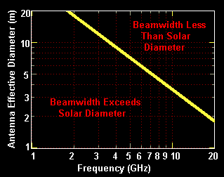
Figure 7 - Antenna beamwidth equals mean solar diameter
3 SATELLITE AND SOLAR POSITIONS
3.1 The Nature of the Problem
The potential for solar interference with a satellite downlink
circuit will occur whenever the Sun passes into the beam
of the ground station receiving antenna. For a geosynchroonous orbit
this will occur around the times of the equinoxes. What we are
interested in are the times and durations of these occurrences,
together with the magnitude of the receiving system temperature
increase that will occur. From this, the degradation in the system
performance is readily determined.
The first problem then is one of determining the position of both
the satellite and the Sun. The former, being relative stationary,
is readily accomplished. The latter, due to the changing length
of our year, orbital variations, and our awkward calendar, is a
little more difficult. Once these positions are obtained we then
need to check for relative coincidences between the two as a function
of time.
The apparent motion of the Sun across the sky renders the normal
elevation-azimuth coordinate system unsatisfactory for use in solving
our problem. Much better is the equatorial system of declination and
hour angle. The Sun in essence then moves in hour angle during a
single day, with a much smaller annual motion in declination. The
equatorial system is based about an axis projected through the poles
to infinity. Hour angle is measured from local meridian (with east
negative) about this axis (in essence celestial longitude), and declination
is measured in a plane containing this axis. Zero declination is
defined at the projection of the equator and angles north of this are
positive (figure 8).
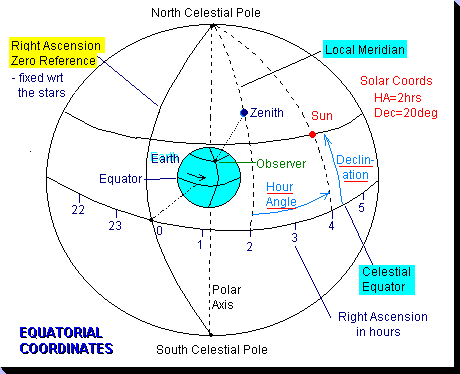
Figure 8 - Equatorial Coordinates
At the equinoxes the solar motion is 0.4 degrees per day in
declination, and thus even with an infinitely small antenna beam, the
Sun will still be in the beam for at least one day per
equinox (figure 9).
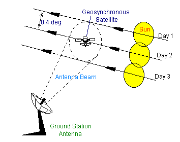
Figure 9 - Transits of the Sun through an antenna
beam on successive days around equinox.
3.2 Satellite Locational Algorithms
For a truly geostationary orbit, the satellite inclination is zero,
and no apparent motion is seen from the ground. If we further allow
the assumption of a spherical Earth, the elevation and azimuth of the
satellite from a fixed ground location (latitude L and longitudinal
difference from the satellite G) are readily given by standard
spherical trigonometrical equations.
The great circle angle T between the satellite and ground station:
Azimuth A:
Elevation e:
tan e = [ (R+h)cosT - R ] / [ (R+h)sinT ] ... eqns 5
where the Earth radius R=6378km and the satellite orbital radius
(R+h) = 42164km.
For completeness, the slant range is given by:
r = sqrt[ R2 + (R+h)2 - 2Rh(R+h)cosT ]
The elevation and azimuth are converted to hour angle (HA) and
declination (δ) through the relations:
Calculations with an oblate Earth model show that the errors incurred
from the spherical approximation amount to around 0.1 degree in
azimuth and elevation and 10km in slant range (at mid-latitudes).
This angular error is one fifth of the solar diameter and less than
many station keeping regimes. In military satellites, which are
often given a considerable non-zero inclination, the errors involved
will be unacceptable, but for most commercial purposes, the
approximation is valid.
3.3 Solar Locational Algorithms
Simple formulae for the solar declination and hour angle are specified
in the Astronomical Almanac (1). The argument of these relations is
a modified Julian day number, including a fraction representing the
time of day. This particular day number is the number of days from
the start of day zero in the year 2000. This can be computed quite
readily using a modification of Sinnot (2) to a single line FORTRAN
algorithm by Fliegel and Van Flandern. The result is expressed
most simply by four lines of BASIC code:
	N=INT(Y+FIX((M-9)/7))
	N=-INT(3*(INT(N/100)+1)/4)
        N=N-INT(7*INT(M+9)/12)+Y)/4
	N=N-730516.5+D+367*Y+INT(275*M/9)         ... eqns 7
where Y is the four digit year (eg 1989), M is the month number (1-12), and D is the day and part day (ie time within the day as a
day fraction) of that month. N may then be used as input to the
following relations (1), which are all expressed using degrees (not
radians!):
	Mean solar longitude L
	  L=280.460+0.9856474*N
	Mean anomaly G
	  G=357.528+0.9856003*N
	L and G must be reduced modulo 360 before substitution in:
	Ecliptic longitude Le
	  Le = L + 1.915*sin(G) + 0.020*sin(2*G)
	Obliquity of the ecliptic e
	  e = 23.439-0.0000004*N
	Right ascension (same quadrant as Le ) RA
	  RA = atan( cos e tan Le )
	Declination dec
	  dec = asin( sin e sin Le )
	The Equation of Time EoT
	  EoT(minutes) = 4 ( L - RA )              ... eqns 8
The equation of time is the time that the Sun is running fast or slow.
That is, local noon will occur at 12.00 - E/60 hours local time. From
this the Hour Angle of the Sun when observed at longitude G0 (degrees
east) is given by:
HA(deg) = 15*( UT - 12 + EoT/60 + G0/15 ) ... eq 9
The term within the parentheses is in hours, which is the more usual
unit for hour angle. However, the use of an angular measure is more
appropriate in this instance. UT is the Universal Time.
If required the apparent angular diameter of the Sun in degrees is
given by:
Πs = 0.534 / (1.00014-0.01671*cos(G) - 0.00014*cos(2*G)) ... eq 10
where the term in parentheses is the normalised Sun-Earth distance.
The accuracy of the declination is 0.01 degree and the hour angle
0.03 degree between the years 1950 and 2050. The hour angle accuracy
corresponds to a timing accuracy of around 10 seconds.
3.4 Range of Coincidence
To find the days on which an effect may occur, the equations (7)
through (8) may be cycled until the solar declination is within a
specified value of the satellite declination. The specified value
is generally taken as half the sum of the antenna beamwidth
(θ = 1.2 λ / de where de is the effective linear aperture)
plus the solar diameter (equation 10 for the higher microwave
frequencies - slightly larger (figure 3) at 1 GHz). On each of
these affected days the equation of time at noon may be used to find
the range of affected times (equation 9). One iteration to find a
corrected EoT will be more than accurate enough for any application.
The greatest inaccuracy lies in selecting the appropriate antenna
contour (eg 3 dB beamwidth) for the computation. This can only be
accurately done after computation of the maximum solar effect on
the given system.
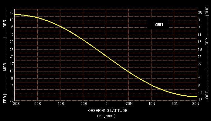
Figure 10 - Dates of maximum solar interference to
satellite signals from geostationary orbit.
4 DOWNLINK CALCULATIONS - CNR CHANGES
4.1 The Central Beam - Depth
The maximum effect will occur if and when the Sun falls centrally
within the antenna response pattern. The appropriate downlink
equation can then be written (neglecting tropospheric attenuation,
etc):
C/N = Pr/(Pn + Psun) = Pt Ae / ( 4πkT(1 + SAe/(kT))Δf r 2) ... eq 11
where T is the system noise temperature. It suffices to note that the
net effect is to raise the effective noise temperature by an amount:
and thus the decrease in the carrier to noise ratio will be given
by:
ΔCNR (dB) = 10 log ( 1 + S Ae / ( k T ) ) ... eq 12
Note that this is independent of operating frequency when expressed
as shown (ie as a function of the system collecting area to
temperature). The more commonly used G/T ratio can be computed from:
G/T = A/T ( 4 π f 2 / c2 )
Table 1 shows the dB decrease in C/N for typical A/T ratios (in dB
metre squared per Kelvin) for the range of solar fluxes typically
encountered from 1 to 20 GHz. Figure 10 shows the same data in terms
of G/T for selected frequencies over a wider range of solar fluxes
which could occur during bursts.
The above formula (eq 12) only holds when the antenna beamwidth
exceeds the solar angular diameter. For a narrow beam system,
the appropriate relationship is:
ΔCNR (dB) = 10 log ( 1 + Tsun / T ) ... eq 13
where Tsun is given by equation 4. The effect of going to equation
13 vice equation 12 is essentially a lowering of the magnitude of
the solar increase. Note that it is preferable to increase A rather
decrease T if a minimal solar effect is desired.
TABLE 1 - C/N decrease (dB) due to solar radio noise

 A/T                        Solar Radio Noise (SFU)
dBm2/K  50  100  150  200  250  300  350  400  450  500  550  600  650  700

-51.0  0.0  0.0  0.0  0.0  0.1  0.1  0.1  0.1  0.1  0.1  0.1  0.1  0.2  0.2
-48.0  0.0  0.0  0.1  0.1  0.1  0.1  0.2  0.2  0.2  0.2  0.3  0.3  0.3  0.3
-45.0  0.0  0.1  0.1  0.2  0.2  0.3  0.3  0.4  0.4  0.5  0.5  0.6  0.6  0.6
-42.0  0.1  0.2  0.3  0.4  0.5  0.6  0.6  0.7  0.8  0.9  1.0  1.1  1.1  1.2
-39.0  0.2  0.4  0.6  0.7  0.9  1.1  1.2  1.4  1.5  1.6  1.8  1.9  2.0  2.1
-36.0  0.4  0.7  1.0  1.3  1.6  1.9  2.1  2.4  2.6  2.8  3.0  3.2  3.4  3.6
-33.0  0.7  1.3  1.9  2.4  2.8  3.2  3.6  3.9  4.2  4.5  4.8  5.0  5.3  5.5
-30.0  1.3  2.4  3.2  3.9  4.5  5.0  5.5  5.9  6.3  6.6  7.0  7.3  7.6  7.8
-27.0  2.4  3.9  5.0  5.9  6.6  7.3  7.8  8.3  8.8  9.2  9.5  9.9 10.2 10.5
-24.0  3.9  5.9  7.3  8.3  9.1  9.8 10.5 11.0 11.5 11.9 12.3 12.6 13.0 13.3
-21.0  5.9  8.3  9.8 11.0 11.9 12.6 13.2 13.8 14.3 14.7 15.1 15.5 15.8 16.2
-18.0  8.3 11.0 12.6 13.8 14.7 15.5 16.1 16.7 17.2 17.7 18.1 18.4 18.8 19.1
-15.0 11.0 13.8 15.5 16.7 17.7 18.4 19.1 19.7 20.2 20.6 21.0 21.4 21.8 22.1
-12.0 13.8 16.7 18.4 19.7 20.6 21.4 22.1 22.6 23.2 23.6 24.0 24.4 24.7 25.1
 -9.0 16.7 19.6 21.4 22.6 23.6 24.4 25.1 25.6 26.1 26.6 27.0 27.4 27.7 28.1
 -6.0 19.6 22.6 24.4 25.6 26.6 27.4 28.0 28.6 29.1 29.6 30.0 30.4 30.7 31.1
 -3.0 22.6 25.6 27.4 28.6 29.6 30.4 31.0 31.6 32.1 32.6 33.0 33.4 33.7 34.0
  0.0 25.6 28.6 30.4 31.6 32.6 33.4 34.0 34.6 35.1 35.6 36.0 36.4 36.7 37.0
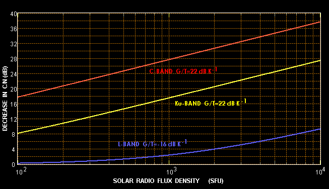
Figure 11 - Showing C/N decrease as a function of solar noise output
for three cases: (1) L-band mobile with G/T = -16 dB/K, (2) C-band 3.5m
aperture with 60 K temp, and (3) Ku band 2.2m aperture with 250 K temp.
4.2 Antenna Polarisation
Solar flux values are reported for the total solar radio output
at a particular frequency. This emission is mostly randomly
polarised, although both left and right hand circular polarisation
burst components are seen around active solar regions with large
magnetic fields. However, the non-burst components are generally
random.
If a receiving antenna has circular polarisation, either left or
right hand, it will receive the full solar flux. If it uses linear
polarisation, however, it will only collect half the reported flux
value, and thus S/2 should be used in all equations instead of the
full flux density S.
4.3 The Peripheral Beam - Duration
The first order calculation of the duration of the solar effect might
use the antenna 3 dB beamwidth. For a central traverse of the Sun
through the antenna, the duration of the effect is then equal to the
sum of the beamwidth (θ) and the solar diameter (Πs) times the
rate of movement of the Sun in hour angle (4 minutes per degree).
Table 2 shows this duration. For an off centre traverse, the time
is given by:
Δt(mins) = 4 cos-1[cos(θ/2 + Πs/2) / cos(Δδ) ] ... eq 14
where the output of the inverse cosine function must be expressed in
degrees, and where Δδ is the declination difference between the Sun
and the antenna beam.
If the solar noise increase is significantly larger than the downlink
C/N margin, then the 3 dB beamwidth may not be appropriate. An
acceptable contour must then be chosen with regard to the fraction
of the solar disc covered by this contour at each moment of the
traverse. Inaccuracies in antenna pointing and errors in the
knowledge of the exact solar output add to the complexity of this
type of calculation.
TABLE 2 - SUN TRANSIT TIME THROUGH ANTENNA BEAM (minutes)

Antenna                 Receiving
Diam                    Frequency (GHz)
 (m)     2    4    6    8   10   12   14   16   18   20

 0.5   86.2 44.3 30.3 23.3 19.1 16.3 14.3 12.8 11.7 10.7
 1.5   30.3 16.3 11.7  9.3  7.9  7.0  6.3  5.8  5.4  5.1
 2.5   19.1 10.7  7.9  6.5  5.7  5.1  4.7  4.4  4.2  4.0
 3.5   14.3  8.3  6.3  5.3  4.7  4.3  4.1  3.8  3.7  3.5
 4.5   11.7  7.0  5.4  4.7  4.2  3.9  3.7  3.5  3.4  3.3
 5.5   10.0  6.2  4.9  4.2  3.9  3.6  3.4  3.3  3.2  3.1
 6.5    8.8  5.6  4.5  4.0  3.6  3.4  3.3  3.1  3.1  3.0
 7.5    7.9  5.1  4.2  3.7  3.5  3.3  3.1  3.0  3.0  2.9
 8.5    7.3  4.8  4.0  3.6  3.3  3.2  3.0  3.0  2.9  2.8
 9.5    6.8  4.5  3.8  3.4  3.2  3.1  3.0  2.9  2.8  2.8
10.5    6.3  4.3  3.7  3.3  3.1  3.0  2.9  2.8  2.8  2.7
4.4 Summary
For a given collecting aperture and noise temperature, the effect
of the Sun on a system increases with frequency (because of the
increasing solar output). Small aperture systems are relatively
unaffected by normal solar noise, although at times of high solar
activity, all satellite downlinks are susceptible, and then small
apertures will be affected for a longer duration. At Ka Band a
relatively small aperture (eg 2m) has a beamwidth less than the solar
diameter and the total solar radio energy collected then starts to
decrease - in most cases, the link margin for tropospheric attenuation
(precipitation) will cope with the solar traverse. In summary, it may
be concluded that moderate apertures at mid-microwave experience the
most significant reduction in carrier to noise ratio (with respect to
the duration-depth product).
The time extent of Sun-outages and their predictability makes it
relatively easy to reduce the limited impact that they cause.
Alternate satellite paths, if available, obviate the problem in most
cases. The one exception may prove to be mobile L-band downlinks.
Very limited aperture and low system noise together with limited link
margins could make these systems quite susceptible to the frequent
solar bursts that occur at times of high solar activity.
5 SOLAR DISTURBANCE TO OTHER SYSTEMS
Any high gain low noise system pointing near the Sun will be subject
to interference. The USA Federal Aviation Authority receives advice
on solar bursts for the aviation emergency channels of 121.5 and
243 MHz. Sun synchronous polar orbiting satellites are particular
liable to experience several consecutive days of passing in front of
the Sun. Military early warning radar is susceptible to 'solar
jamming'. Historically, solar radio emissions were first recognised
as such through jamming of the British coastal home chain
radars during World War II.
6 THE SUN AS A CALIBRATION SOURCE
In the inverse of the problem just discussed, a known solar radio
output on a specific frequency may be used to measure the G/T of a
microwave receiving system.
The sun is allowed to drift through the antenna beam, and the increase
in noise power is determined. This is most accurately accomplished
through the use of an attenuator in the RF line to reduce the peak
solar noise back down to the level of the normal system noise. This
noise power increase β(dB) may then be used to determine the system
G/T through the expression:
G/T (dB) = 10 * log [ 4 π k (10β/10 - 1) / ( λ2 S) ] ... eq 15
The only precaution to be taken in this measurement is to make sure
that any burst component is absent. Two successive measurements,
equal within experimental error will suffice to establish this
condition. IPS Radio and Space Services in Australia can provide
near real-time values of solar flux and advise on burst activity.
Remember that if the antenna under test is linearly polarised then
the value of solar flux S should be reduced by 50%.
7 REFERENCES
- Anawalt RA and A Boksenberg, The Astronomical Almanac 1989,
USGPO (Washington) & HMSO (London), 1988
- Sinnot RW, "Taming Our Chaotic Calendar", Sky and Telescope,
v70(#5), pp454-455, 1984
- Smerd SF, Annals of the IGY, v34, 1964
- Kundu MR, Solar Radio Astronomy, Wiley (New York), 1965
- US Department of Commerce, Solar Geophysical Data, various
issues, Boulder Colorado, 1988
Australian Space Academy
 Home
Home