 |
 |
cause photometric errors. |
single satellite trail. |
Note: The material presented here was originally published in the Proceedings of the Australian Space Research Conference 2017
SUMMARY
The increasing space debris population can cause problems both to space systems and to systems on the ground. One of the latter problems is the presence of increasing numbers of satellite and debris trails across astronomical imagery. The effects of this pollution can range from errors in automated photometry systems to cosmetic rejection. To evaluate the extent of this problem we have used the Hough transform to detect satellite trails in large astronomical image databases.
INTRODUCTION
The increasing space debris population can cause problems both to space systems and to systems on the ground. One of the latter problems is the presence of increasing numbers of satellite and debris trails across astronomical imagery. The effects of this pollution can range from errors in automated photometry systems to cosmetic rejection. To evaluate the extent of this problem we have used the Hough transform to detect satellite trails in large astronomical image databases.
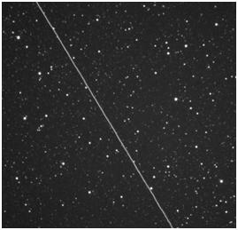
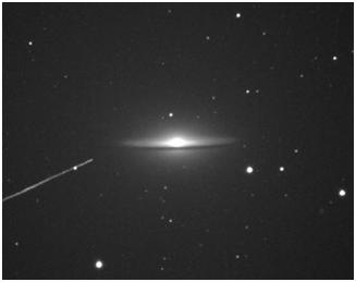
There have been typically two issues with contamination of astronomical imagery from satellites: errors in photometry and degradation due to aesthetic quality of the image. Figures 1 and 2 show examples of both of these cases.
|
|
cause photometric errors. |
single satellite trail. |
Various authors have discussed the problem of satellite trails in images previously, mostly with an aim of rejecting corrupted images from automated processing pipelines. Storkey et al [2] and Stöveken and Schildknecht [3] discuss a variety of techniques for removing satellite trails and other artifacts from sky surveys. Borncamp and Lim [4] describe their technique for removing satellite contaminated images from surveys using the Hough transform.
In our work, we also use the Hough Transform to identify images of satellite trails. We developed an algorithm that analysed over 45000 images from the Perth Observatory Skynet Telescope [5]. Our aim in this analysis is to try and quantify the problem and set a baseline for future studies to follow the progressive effects of increasing numbers of space objects in Earth orbit.
The remainder of this paper discusses the Hough Transform, its implementation for detecting satellite trails and the results of our analysis.
THE HOUGH TRANSFORM
The Hough Transform was originally developed and patented by Hough in 1962 [6]. Duda and Hart modified and implemented the Hough Transform in 1972 [7]. The Hough Transform is able to detect linear (and other) features in an image. It has not been widely utilised until recently as it is computationally intensive. With the increase in computer capability, this transform is being applied more widely. For the full details of the Hough Transform, refer to the lecture notes by Solberg [8], but a summary is provided here.
Pre-processing
Typically before lines in an image can be found, an edge detection filter (such as a Sobel filter) is applied to the image in order to produce a black and white image with only edges in it. In the case of astronomical images with satellite trails, often the edges are not well defined. In addition the thickness of the trail can vary significantly, making it difficult to determine a threshold for edges.
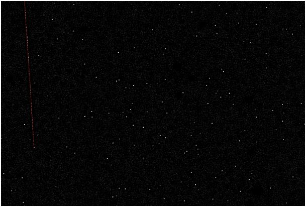
Rather than using edge detection, our algorithm uses neighbourhood pixels to determine if a pixel may potentially be on a line. Consider figure 3, where the satellite trail is a near vertical line on the left of the image.
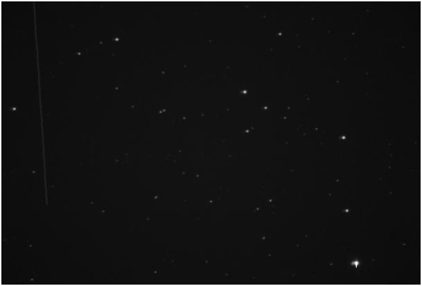
To convert this into a black and white image, the mean (μ) and standard deviation (σ) of the pixel intensities of a 21 by 21 pixel box surrounding each pixel is found. A threshold intensity value (T) is determined by Eqn 1:
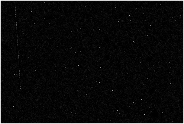
If the pixel at the centre of the box exceeds T, then it is marked as 1, otherwise 0. This process is performed for each pixel in the image. In addition bright pixels (such as those of the star at the bottom right of Fig. 3) are omitted. Figure 4 shows the resulting binary image.
The Hough Transform
A single point [x,y] in an image can have many lines going through it. For any given line through this point, we use the polar representation for the line, Eqn 2:
This representation is shown in Figure 5.
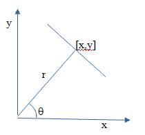 |
Fig. 5: Polar Representation of a Line. The line from the origin to [x,y] intersects the line at right angles and has distance r and angle θ from the x-axis. |
With this definition of a line, r has a range from +R to -R where:
where xs and ys are the size of the x-axis and y-axis respectively, and the angle θ can range from -π/2 to +π/2. A particular point in an image is restricted to certain values in [r,θ] space, as shown in Figure 6.
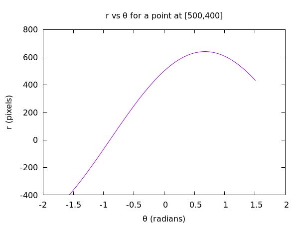
Fig. 6: Example θ vs r plot for a point on an image.
The [r,θ] values for each point form a sine curve.
If two points lie on the same line, their [r,θ] curves will intersect at the [r,θ] value that they have in common. The Hough Transform then proceeds as follows:
2. Create an array of size rn by θn, where rn is the number of r values and θn is the number of θ values. This array is an accumulator, effectively a 3 dimensional histogram.
3. For each pixel, loop through each θ value. Compute r for each θ value and select the nearest discrete r value.
4. Increment by one the appropriate [r,θ] element in the accumulator. The more counts an element has in the accumulator, the more points there are on that particular line.
5. Figures 7 and 8 shows the accumulator associated with Figure 4.
6. If the number of counts in a particular element exceeds a certain value, then the [r,θ] value associated with that element is considered to be a line in the image. We used a six sigma detection for our threshold value.
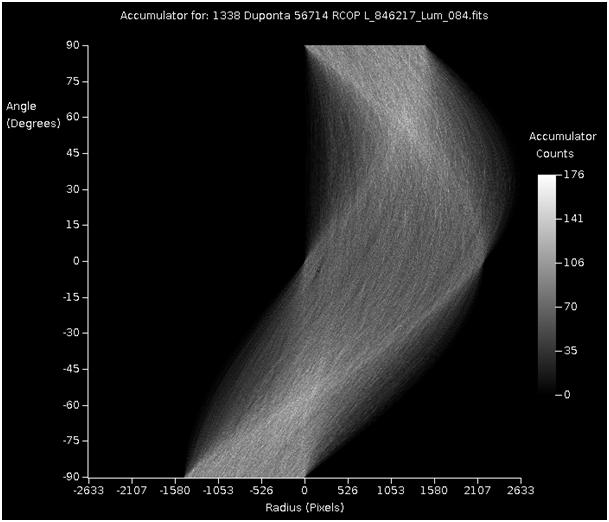
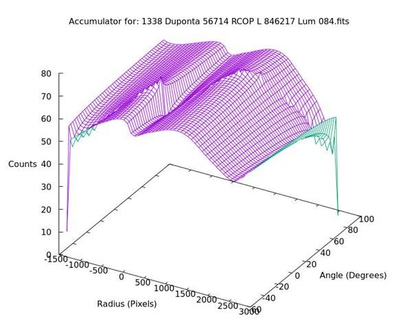
Unfortunately, retrieving the lines is not so straightforward. The satellite trails are usually more than one pixel wide, thus leading to multiple lines which sit about the ‘true’ satellite trail. In addition, typically the bins in the accumulator around the ‘true’ satellite trail [r,θ] value also exceed our threshold. In the above example there were 79 lines associated with the single satellite trail.
To overcome this problem, only peaks in the accumulator were considered. This reduced the number of lines to 7. To obtain the single line, the number of marked pixels along each line was computed. The line that had the most number of marked pixels was used as the satellite trail line.
The Hough Transform only gives the equations for the lines in the image, not the start and end points of the line. To obtain the start and end of the line, pixels are examined along the path of the line. Continuous line segments are found, and combined to produce the final line. The line width is also determined by finding pixels that are marked which are adjacent to the line. Once this process is complete the line is removed from the binary image and the Hough transform repeated to determine if there are any more lines in the image. Figure 9 shows the detected satellite trail from figure 4 marked in red.
RESULTS
Initially about 45,000 FITS images from the 35cm Skynet Telescope located at Perth Observatory were analysed. From the header on each image, the following values were extracted: the date and time of the image, the exposure time, the central declination and right ascension of the image, and the filter employed. To this was added the filename of the image and the calculated total area covered by the image (this was essentially fixed by the telescope field of view). After the image had been processed, the total number of detected satellite trails was appended. Where this number was non-zero, additional information was added about each trail. This consisted of the length of the trail in pixels, the width of the trail in pixels, and the angle of the trail with respect to the x-axis of the image. All these records were then stored in a single file per telescope for subsequent statistical analysis. Initial analysis was made of a large number of images from the Skynet telescope located at the Perth Observatory. This is a robotic telescope operated for the University of North Carolina. Table 1 shows the telescope parameters:
|
APERTURE: 0.35 m FOCAL LENGTH: 2000.0 mm F-RATIO: 5.6 FILTERS: B,V,R,I, Halpha, OIII, Open, SPEC100 CCD SIZE: 2184 x 1472 (6 um pixels) FOV: 25.5 x 17.2 arcmins |
The images analysed were acquired during the period 2013 to 2014. Analysis of detected trails with declination are given in table 2. The declination range is a combination of both southerly and northerly declinations. This is done because satellite orbits are symmetric. However, as the telescope does not observe above declination +40 degrees, all the trails from 40 to 90 degrees come from southerly declinations. In total 4.1% of the images displayed satellite trails. The large number of images in the declination range from 60 to 69 degrees comes from a project which was frequently observing the massive star Eta Carina during the analysis period. Apart from this the decreasing number of images with increasing declination simply represents the decreasing sky area as the declination tends toward the poles.
| Declination (θ) | # Images | # Trails | %Trails |
| 00 - 09 | 6237 | 1736 | 27.83 |
| 10 - 19 | 6570 | 37 | 0.56 |
| 20 - 29 | 4508 | 10 | 0.22 |
| 30 - 39 | 2022 | 9 | 0.45 |
| 40 - 49 | 1034 | 0 | 0.00 |
| 50 - 59 | 537 | 2 | 0.37 |
| 60 - 69 | 23127 | 27 | 0.12 |
| 70 - 79 | 409 | 0 | 0.00 |
| 80 - 89 | 4 | 0 | 0.00 |
| 00 - 89 (Total) | 44448 | 1821 | 4.10 |
The data given in Table 2 is essentially raw data. To be useful for comparisons in the future and with different instruments we need to take into account the exposure time for each image and the area of sky covered. For the Perth Skynet telescope each exposure covers 389 square arc minutes of sky. Table 3 gives the detailed results of this analysis. Total exposure time was 1,724,489 seconds and the average detection rate was 35.2 trails per square degree per hour.
_____________________________________________________________________
|                                                                   |
| Declination Exposures     Trails       %Time    Num/hour  Detrate |
|  (degrees)  (num/time) (num/exptime)  /%Trails                    |
|                                                                   |
| 00 - 09   6237/413920   1746/9218    2.23/27.83   15.10    139.7  |
| 10 - 19   6570/463034     37/2970    0.64/0.56     0.29      2.7  |
| 20 - 29   4508/182129     10/610     0.34/0.22     0.20      1.8  |
| 30 - 39   2022/103209      9/660     0.64/0.44     0.31      2.9  |
| 40 - 49   1034/23632       0/0       0.00/0.00     0.00      0.0  |
| 50 - 59    537/28927       2/130     0.45/0.37     0.25      2.3  |
| 60 - 69  23127/479694     27/972     0.20/0.12     0.20      1.9  |
| 70 - 79    409/29464       0/0       0.00/0.00     0.00      0.0  |
| 80 - 89      4/480	     0/0       0.00/0.00     0.00      0.0  |
|___________________________________________________________________|
The above analysis does not include a sensitivity factor due to telescope aperture, f-ratio, filter or CCD camera sensitivity.
DISCUSSION
All 1821 images in which a trail was found automatically were examined visually. In quite a few images the trail was so faint that it could be detected by eye only with great difficulty. We can thus state that our implementation of the Hough transform was able to extract very faint satellite trails. The error rate with the thresholds used was very low. These few misdetections were manually excluded from the subsequent analysis, but would not have greatly affected the statistics had they not been so removed.
Examination of satellite trails by declination shows that most of the satellite trails are due to geosynchronous objects, despite the greater brightness of the closer low Earth orbit objects. This is due to the much greater angular speed of objects in low Earth orbit. Such objects would in general cross the field of view in a time substantially less than the exposure time, whereas geosats will normally be present for almost the entire exposure, unless they are at the edge of the image.
Geostationary satellites (those with near zero inclination) will only be found in the lowest declination range. The exact declination will depend on the latitude of the observing station. For Perth, geostationary satellites lie within a degree of +5 degrees declination (the exact value varies with the hour angle of the satellite). Geosynchronous satellites on the other hand, although they still have an orbital period of 1436 minutes (synchronous with the Earth's sidereal rotational period), they may have an orbital inclination of up to or exceeding 30 degrees. Most active geosats however, with the exception of some military satellites, usually have inclinations of less than 10 degrees. At the end of life a geosat will normally be placed in a supersynchronous orbit (>300km above geosynchronous orbit). Such pieces of debris will still produce long exposures on astronomical images. Because of the increasing proliferation of geosynchronous and supersynchronous objects all clustered moderately tightly around equatorial declinations the probability of finding more than one trail on a single exposure is not uncommon. This is almost never the case for low Earth objects.
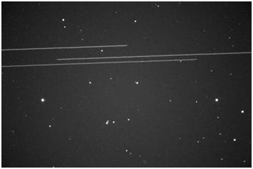
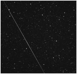
All detections were examined visually and only one was found to be a possible meteor. Figure 9 shows an example of multiple trails in an image and figure 10 shows a possible meteor trail.
 |
 |
| Figure 9: One in four images in a 20 degree band around the celestial equator will contain a trail due to a geosynchronous satellite. Multiple trails may occur. |
Figure 10: Of all the 1821 detected trails this is the only one that appears more likely to be natural space debris (ie a meteor). |
When normalised for exposure time and sky area covered, the average detection rate of space debris (including active satellites) for the Perth Skynet telescope (32 cm aperture) is 35 per square degree per hour. This can be broken down to an average detection rate of low Earth orbiting objects of around 2 trails per square degree per hour (across the whole sky) and a detection rate for geosats of nearly 140 trails per square degree per hour in a 20 degree declination band centred on the celestial equator. The detection rate for natural space debris (meteors) is very roughly one thousand times less than that for artificial space objects, with a best estimate of around 0.02 meteors per square degree per hour. For comparison with other telescopes at future times a system sensitivity factor must be considered. This will involve the telescope aperture, focal length, mirror efficiency, filter and camera efficiency. Although exact quantification of all these effects is not an easy matter, it is planned to perform further work with image datasets from other telescope systems to provide rough guidelines toward such a sensitivity factor that can be used to provide an overall normalised detection rate. With such a normalised rate, we hope that it will be possible to monitor and provide a quantitative estimate of the progressive growth of this phenomenon into the future.
ACKNOWLEDGEMENTS
Acknowledgement is made to Dan Reichart, Univ of North Carolina, for the Skynet Robotic Telescope Network, and to Arie Verveer for providing the images used in this analysis.
REFERENCES
1. Lovell, B., "The Challenge of Space Research", Nature, Vol 195, pp 935ff, 1962.
2. Storkey, A. J., Hambly, N. C., Williams, C. K. I. and Mann, R. G, “Cleaning Sky Survey Databases using Hough Transform and Renewal String Approaches”, Monthly Notices of the Royal Astronomical Society, Vol 347, Issue 1, 2004, pp 36 -51.
3. Stöveken, E. and Schildknecht, T., “Algorithms for the Optical Detection of Space Debris Objects”, Proceedings of the Fourth European Conference on Space Debris, Darmstadt, 18-20 April 2005.
4. Borncamp, D. and Lim, P. L., “Satellite Detection in Advanced Camera for Surveys/Wide Field Channel Images”, Instrument Science Report ACS 2016-0, 2016.
5. Skynet Robotic Telescope Network, < https://skynet.unc.edu/>[Accessed 14 Dec 2018]
6. Hough, P. V. C, “Hough Method and Means for Recognizing Complex Patterns”, US Patent Number 3069654 A, 1962.
7. Duda, R. O. and Hart, E. H., “Use of the Hough Transformation to Detect Lines and Curves in Pictures”, Communications of the ACM, Vol 15, Issue 1, 1972, pp 11-15.
8. Solberg, A. (2009). INF 4300 Lecture Notes. Available at: https://www.uio.no/studier /emner/matnat/ifi/INF4300/h09/undervisningsmateriale/hough09.pdf [Accessed 17 Jan 2018].
 Australian Space Academy